A few readers may be interested in how I used Stata to create the color scheme for the offenses in the graphs I’ve posted recently. This is a “stats nerd” post that assumes the reader uses Stata, a statistical package. Everybody else may wish to give it a pass. Some preliminary tricks, then the code. UPDATED 8/6/2017 to include RGB values in the color palette and to give the formulas for calculating them from intensities.
Trick 1 that I have learned is to generate self-labeling lines by creating a variable that has the label only in the last value of the x-axis variable, year in my case. E.g. gen xvalue15=Label if xvalue==15. Or self-labeling scatterplots by having a label for all values.
Trick 2 is to use Stata macros to generate the lines of a plot. The general scheme is:
local plotlist ""
foreach val in `list of values' {
    local plotlist "`plotlist' (code_for_one_line )"
    }
twoway `plotlist', [code for graph as a whole]
In this code, each line gets added to the macro plotlist. Pro tip: remember to reset the plot macro to ” ” (empty) (or use a new macro name each time) or you will get unpleasant results with repeated graphs.
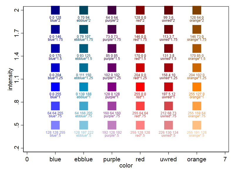
Color Swatch Generator
Although Stata can generate colors using any set of RGB values, for a variety of reasons* I found it easiest to work with the built-in named colors. Named colors can be modified with the syntax “color*##. Numbers less than 1 lighten the color and numbers greater than 1 darken the color. The ado file full_palette generates a swatch of the 66 named colors in Stata, with their RGB values (you can access this by typing help full_palette and installing the ado), and the built-in ado palette color will show color samples and the RGB values for two colors (type help palette color to see the syntax of the command). But I wanted to see ranges of colors using the intensity values across several different named colors. I also tested creating my own color (uwred) and saving it in a .style file. **
* Stata program to generate color swatches
* Pamela Oliver 5/29/2017, updated 6/18/2017 and 8/6/2017
* now locates .style file for named color and identifies RGB code
* calculates and prints RGB values as well as color names
* uses syntax "scatter y1 y2 x" to  print two-line labels
* edits code so colors now print in the order of colorlist
     * instead of alphabetical
* uwred is a color I created and saved in my personal ado file
version 14.2
local colorlist "ebblue eltblue orange orange_red red uwred purple"
local intenlist ".8 1 1.3 1.5 1.8 2"
local intnumlist=subinstr("`intenlist'"," ",", ",.) // a numlist with commas
disp "`intnumlist'"
** This code to get a decent intensity range in the graph regardless of entries
local maxint=max(`intnumlist')
local minint=min(`intnumlist')
disp `maxint' `minint'
local range=`maxint'-`minint'
local edgegap=round(`range'*.2,.01)
local labgap=`edgegap'/8
local lowint=`minint'-`edgegap'
local yrange "`lowint' (`edgegap') `maxint'"
** This code generates the data for the plots
local ncolor=wordcount("`colorlist'")
local ninten=wordcount("`intenlist'")
local ncases=`ncolor'*`ninten'
disp "ncolor `ncolor' ninten `ninten' ncases `ncases'"
set more off
clear
set obs `ncases'
gen case=_n
gen ncases=_N
gen color=""
gen intenS=""
gen colorname=""
** fill in the strings with colors and intensities
local ii=1
forval color= 1/`ncolor' {
forval inten= 1/`ninten' {
     replace basecolor=word("`colorlist'",`color') if case==`ii'
     replace colornum=color' if case==ii'
 replace intenS=word("`intenlist'",`inten') if case==`ii'
 replace colorname=color+"*"+intenS
 replace col_int_num=ii' if case==ii' local ii=`ii'+1 } }
*** the num variables are sequential
** uses the string variables as value labels for the numerical variables
labmask colornum, values(basecolor)
labmask col_int_num, values(colorname)
** create numeric version of intensity
encode intenS, gen(intennum)
gen inten=real(intenS) // this is the actual numeric value of intensity
gen RGB_base=""
gen RGB_base=""
** this code snippet taken from full_palette.ado with modifications
** it finds and reads the color style file for each named color
** and extracts the RGB values for that color and puts it in a variable RGB_base
** I did not copy all the error code returns
foreach base in `colorlist' {
 tempname hdl`base'  // assigns a tempfile name
 findfile color-`base'.style // this command searches all ado directories
 local colorfile=r(fn)  // findfile returns the file location
 file open `hdl`base'' using "`colorfile'", read text
 file read `hdl`base'' line
 while r(eof)==0 {
 tokenize `"`line'"'
 if "`1'"=="set" & "`2'"=="rgb" {
 *qui replace lab=`""`3'`basemod'""' in `i'  // the code from full_palette.ado
 qui replace RGB_base="`3'" if basecolor=="`base'"
 file close `hdl`base'' continue, break
 }
 file read `hdl`base'' line
 }
 }
*** parse the original RGB codes
gen Ro=real(word(RGB_base,1))
gen Go=real(word(RGB_base,2))
gen Bo=real(word(RGB_base,3))
foreach CC in R G B {
 gen `CC'x=`CC'o if inten==1
 replace `CC'x=round(`CC'o/inten,1) if inten>1
 replace `CC'x=`CC'o + round((1-inten)*(255-`CC'o)) if inten<1
 }
gen RGB_derived=string(Rx)+" "+string(Gx)+" "+string(Bx)
** gen a value of inten just a little lower to carry the second label
gen int2=inten-`labgap'  // slightly lower value on vertical axis
set scheme s1color
local plot ""
local plot2 ""
summ col_int_num
local nplots=r(max)
forval point=1/`nplots' {
 **get the values for each point in the plot
 qui summ col_int_num if col_int_num==`point'
 local labelnum=r(mean)
 local colorname: label col_int_num `labelnum'
 qui summ colornum if col_int_num==`point'
 local colnum=r(mean)
 local color: label colornum `colnum'
 qui summ intennum if col_int_num==`point'
 local intnum=r(mean)
 local inten: label intennum `intnum'
** collect the plots for each point in locals named plot and plot2
 local plot "`plot' (scatter inten colornum if col_int_num==`point', mcolor(`colorname') msize(huge) mlab(colorname) mlabc(`colorname') mlabsize(tiny) mlabpos(6))"
 local plot2 "`plot2' (scatter inten int2 colornum if col_int_num==`point', ms(S none) mcolor(`colorname' `colorname') msize(*3 *3) mlab( RGB_derived colorname) mlabc(`colorname' `colorname') mlabsize(vsmall vsmall) mlabpos(6 6))"
 } // end of the loop defining the plots
*disp "`plot'" // in case you need to check whether it worked
local xmax=`ncolor'+1 // put an extra column of padding in the table
local testname "test_today" // give a unique name to the output file
** plot with just the colornames and round swatches
twoway `plot' , legend(off) ylab(.25 (.25) 2) xlab(0 (1) `xmax', val) xtitle(color) ytitle(intensity)
graph export `testname'_sample_color_swatch.png, replace
**plot with two labels and square swatches
twoway `plot2' , legend(off) ylab(`yrange') xlab(0 (1) `xmax', val) xtitle(color) ytitle(intensity)
graph export `testname'_color_swatch_RGB2.png, replace width(800) height(600) exit
Color Line Generator
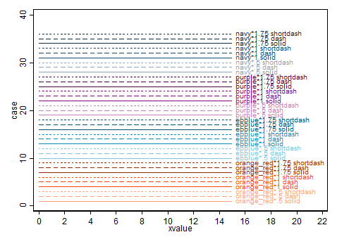
My application has too many values to use just color (or so I judged) so I also used line type. Thus the code to generate sample lines.
stata 14.2
* insert colors, intensities, patterns in the lists as desired

local colorlist "orange_red ebblue"
local intenlist ".5  1 1.75 "
local lplist "solid dash shortdash"
local ncolor=wordcount("`colorlist'")
local ninten=wordcount("`intenlist'")
local nlp = wordcount("`lplist'")
local ncases=`ncolor'*`ninten'*`nlp'
clear
set obs `ncases'
gen case=_n
gen Ncases=_N
gen hue=""
gen inten=""
gen linepat=""
set more off
set scheme s1color  // white background
*** fill in the color values, text variables
local xx=1
forval col=1/`ncolor' {
     forval int=1/`ninten' {
       forval lpat=1/`nlp' {
          replace hue=word("`colorlist'", `col') if case==`xx'
          replace inten=word("`intenlist'", `int') if case==`xx'
          replace linepat=word("`lplist'", `lpat') if case==`xx'
       local xx=`xx'+1
       }
       }
       }
** CREATE 16 values for the X axis ******
Duplicate observations
expand 2, gen(copy1)
expand 2, gen(copy2)
expand 2, gen(copy3)
expand 2, gen(copy4)
gen xvalue=copy1 + 2*copy2 + 4*copy3 + 8*copy4

* generate text from other text
gen color=hue+"*"+inten
gen definition=hue+"*"+inten+" "+linepat
gen def15=definition if xvalue==15
* create numeric variables with the strings as values
encode color, gen(colornum)
encode linepat, gen(lpnum)
qui sum colornum
local ncol=r(max)
forval colnum=1/`ncol' {
    local col`colnum' = `colnum'
    }
forval lpnum=1/`nlp' {
     local lp`lpnum'=`lpnum'
    }

local plotlist ""
disp "ncases `ncases'"
forval case=1/`ncases' {

    qui summ colornum if case==`case'
    local cn=r(mean)
    local color: label colornum `cn'

    qui summ lpnum if case==`case'
    local ln=r(mean)
    local lpat: label lpnum `ln'

    local plotlist "`plotlist' (connected case xvalue if case==`case', msym(i) mlab(def15) lc(`color') mlabc(`color'') lp(`lpat'))"
    }
twoway `plotlist', legend(off) xlab(0 (2) 22)
graph export color_lines_sample.png, replace
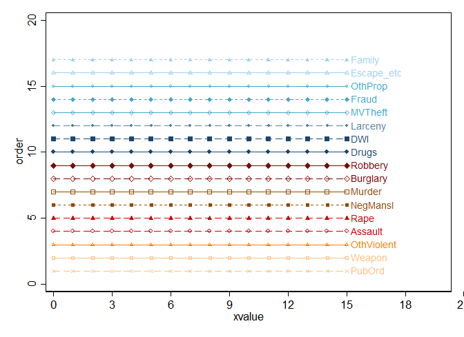
Offense line palette
This is the problem that started me on this path. I have 17 offenses for which I want to graph imprisonment over time. Letting Stata choose the colors generates an unreadable hash. And brewscheme won’t help because I want to assign particular markers/colors to particular offenses, not create a general order of colors. After working on this problem a while, I realized the graph could be more meaningful if similar offenses had related colors. Generating a variable-specific palette is easy using the skills developed above.
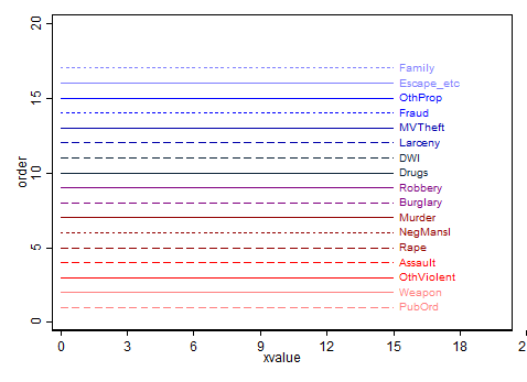
Step 1: Create a spreadsheet with the variable names and labels plus columns for variable groups, color name (hue), intensity, line type, and the order in which I wanted the graphs to appear in my sample. This last is to put the colors that might be difficult to distinguish next to each other in the sample. In my spreadsheet, I put different possible color schemes in different tabs. Here is one sample.
| OffLab | offdetail | group | hue | intensity | line | order |
| Drugs | 12 | drugdwi | navy | 2 | solid | 10 |
| DWI | 20 | drugdwi | navy | 2 | dash | 11 |
| Escape_etc | 21 | misc | ebblue | 0.5 | solid | 16 |
| Family | 22 | misc | ebblue | 0.5 | shortdash | 17 |
| Larceny | 8 | property | ebblue | 1.5 | dash | 12 |
| MVTheft | 9 | property | ebblue | 1.5 | solid | 13 |
| Fraud | 10 | property | ebblue | 1 | shortdash | 14 |
| OthProp | 11 | property | ebblue | 1 | solid | 15 |
| Robbery | 4 | robbur | purple | 1 | solid | 9 |
| Burglary | 7 | robbur | purple | 1 | dash | 8 |
| Murder | 1 | violent | orange_red | 1.75 | solid | 7 |
| NegMansl | 2 | violent | orange_red | 1.75 | shortdash | 6 |
| Rape | 3 | violent | orange_red | 1.75 | dash | 5 |
| Assault | 5 | violent | orange_red | 1 | dash | 4 |
| OthViolent | 6 | violent | orange_red | 1 | solid | 3 |
| Weapon | 23 | violent | orange_red | 0.5 | solid | 2 |
| PubOrd | 13 | violent | orange_red | 0.5 | dash | 1 |
The do file reads the spreadsheet (with a local parameter that selects the tab) and generates a sample plot.
stata 14.2
local group set1
import excel "offense_colors_lines.xlsx", sheet("`group'") firstrow allstring clear
gen color=hue+"*"+intensity
encode color, gen(colornum)
encode line, gen(linenum)
destring offdetail, replace
destring order, replace

** I save this as a Stata file so I can merge it into the data file for production runs

save "offense_lines_2017-6-1`group'.dta", replace

levelsof offdetail, local(offlist) clean
foreach off in `offlist' {
    qui summ colornum if offdetail==`off'
    local cnum=r(mean)
    local col`off': label colornum `cnum'
    qui summ linenum if offdetail==`off'
    local lnum=r(mean)
    local line`off': label linenum `lnum'
    }
** creates values for an X axis
expand 2, gen(copy1)
expand 2, gen(copy2)
expand 2, gen(copy3)
expand 2, gen(copy4)
gen xvalue=copy1 + 2*copy2 + 4* copy3 + 8*copy4
gen OffLab15=OffLab if xvalue==15


local plotlist ""
forval xx=1/17 {
   qui summ offdetail if order==`xx'
   local off=r(mean)
   local plotlist "`plotlist' (connected order xvalue if offdetail==`off', ml(OffLab15) ms(i) lc(`col`off'') mlabc(`col`off'') lp(`line`off''))"
    }
disp "`plotlist'"
twoway `plotlist', legend(off) xlab(0 (3) 20)
graph export "offense_lines_2017-6-1`group'.png", replace
Using this scheme in my production graphs involves this code:
use [data file]

merge m:1 offdetail using offense_lines_2017-6-1set1.dta

levelsof offdetail, local(offlist) clean
foreach off in `offlist' {
     qui summ colornum if offdetail==`off'
     local cnum=r(mean)
     local col`off': label colornum `cnum'
     qui summ linenum if offdetail==`off'
     local lnum=r(mean)
     local line`off': label linenum `lnum'
     }
These local macros can then be used in the production graphs with the same code logic as was used to generate the samples.
Notes
Originally blogged at:
Stata: roll your own color palettes
* I originally tried to use the RGB values from specific palettes I found on line, but passing RGB values in a macro the way I do with my offense colors did not work. I think the problem is a subtle Stata bug/behavior about parsing quotes within quotes within quotes in macros referring to macros and/or the parsing of a list of numbers separated only by spaces. When I used the most straightforward syntax, Stata eliminated the spaces between the numbers (a very odd behavior!), and when I added the Stata special double quotes `” and “‘ , that problem was solved but the resulting code generated an error. However, if you use ado files you can find on line to create and save new colors with names, those new colors should work fine with this routine. You create a new color by creating a file named color-COLORNAME.style in your personal ado path (I put it in a style folder that had previously been created but anywhere works); the content of this file must be
set rgb "255 255 255"
where you replace the 255’s with the RGB codes for the color you want to name. If you examine the color-NAME.style files in your system files (which you can find by typing “findfile color-red.style” in a Stata session and reading the resulting path) you will see that you can also include comments labels and other commands that don’t get in the way of this core command, but this is the one you need.
** I spent some time studying the code for the ado files palette.ado and full_palette.ado trying to figure out how the RGB values were generated from the color and intensity values so I could put them in my palette as well, but finally gave up. Both ado files read the RGB code for the base color from the color .style file, but I could not find the code in palette.ado that computes the derived RGB when there is an intensity factor. It must not look the way I’m expecting it to look.
By experimentation with putting values into palette color, I learned that an intensity greater than 1 consistently divides the RGB values by that number (e.g. ebblue is RGB 0 139 188 and ebblue*2 is 0 70 94). Lower RGB values are darker with black being 0 0 0). An intensity less than 1 increases the values of all three RGB values and pulls it toward white, which has RGB 255 255 255. So for example, red is 255 0 0 , red*5 is 255 128 128, red*.2 is 255 204 204, ebblue is 0 139 188, ebblue*.5 is 128 197 222, teal is 110 142 132, teal*.5 is 183 199 194, teal*.2 is 226 232 230. If the color is pure and fully saturated, the intensity factor adds (1-int)*255 to the other colors. I am sure I could empirically work out the formula for intensities less than 1 for the more complex cases if I spend more time on it, but it is not immediately obvious to me. If you know the formula and put it in the comments, I would be grateful. I’m not sure it matters except to my curiosity. EDIT: The correct general formula for intensity<1 is: orig_RGBnum + (1-intensity)(255-orig_RGBnum) for each of the three original RGB numbers. I still have not found the actual code that implements these formulas in the palette.ado file. But I was able to implement the formula in my own program.