Stata for Students: Basic Statistics, Regression and Graphs
Stata is a popular statistical program at the SSCC that is used both for research and for teaching statistics. Stata for Students is focused on the latter and is intended for students taking classes that use Stata. Those who plan on doing research with Stata should read the more rigorous introduction found in Stata for Researchers.
Stata for Students has two parts: Using Stata and Basic Statistics, Regression and Graphs. You may want to read Using Stata at the beginning of the semester and then read Basic Statistics, Regression and Graphs as your class covers its topics.
Basic Statistics, Regression and Graphs covers the following topics:
The best way to read Basic Statistics, Regression and Graphs is probably to wait until your class covers a topic and then read the matching section.
Stata comes with a sample data set of cars from 1978 which we'll use in the examples in this article. Open it by clicking File, Open, the C: drive, Program Files (x86), (or just Program Files on some computers) then Stata14 and finally double-click auto.dta. Alternatively you can type:
use "C:\Program Files (x86)\Stata14\auto"
or
use "C:\Program Files\Stata14\auto"
or, if you run into problems with these commands, just:
sysuse auto
Basic Statistics
Stata has a large number of commands dedicated to basic statistics; we'll discuss some of the most commonly used. Feel free to skip any you don't need.
Summary Statistics
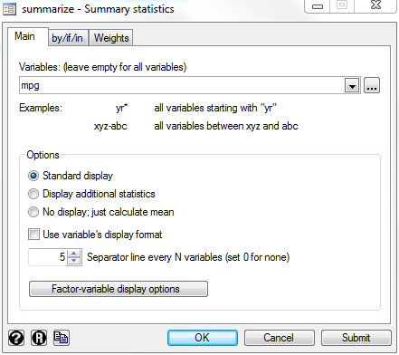
The basic summarize command gives you number of observations, means, standard deviations, minimums and maximums. To use it, click Statistics, then Summaries, tables, and tests, then Summary and descriptive statistics and finally Summary statistics. Select or type mpg in Variables, then click Submit.
Alternatively, you could have just typed:
sum mpg
and gotten the exact same thing (sum being an abbreviation for summarize).
Missing values are ignored when calculating summary statistics. If you type:
sum rep78
you'll see that the number of observations is 69 rather than 74 like it was for mpg. Five observations have missing values for rep78 and could not be included in the calculations, so the mean was calculated over the 69 observations that do have valid values.
Variable lists, if conditions, by groups and options work for summarize just like they did for list in the examples in part one. You've already seen a variable list in action (getting summary statistics for mpg or rep78 rather than all variables). Next, find the mean of mpg for cars weighing over 4,000 pounds by clicking by/if/in and typing weight>4000 in the If box.
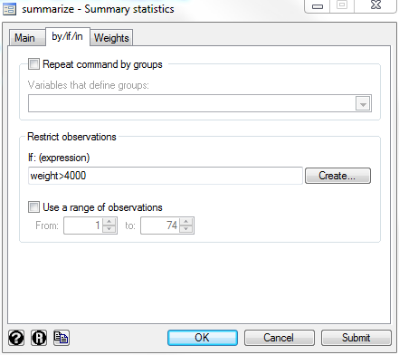
The command for this is:
sum mpg if weight>4000
Now find the mean mpg of the domestic cars and the foreign cars separately: remove the If condition, check Repeat commands by groups, and type or select foreign in Variables that define groups.
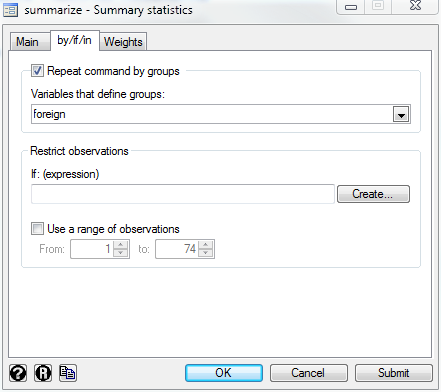
The resulting command is:
by foreign, sort: sum mpg
Finally, there is an option to display additional statistics, like percentiles (including the 50th percentile, better known as the median). Uncheck the Repeat commands by groups box, click on the Main tab, and select Display additional statistics.
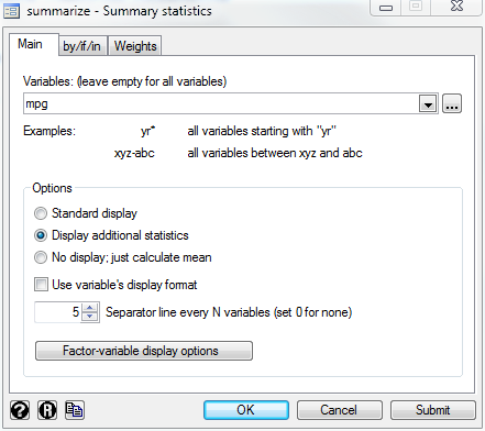
The resulting command is:
sum mpg, details
Frequencies
The tabulate command is used to create frequency tables. It has two variants: one for one-way tables and one for two-way tables. If you type tab, Stata will figure out version which you want by looking at how many variables you list afterwards. But if you're using menus you'll click Statistics, Summaries, tables, and tests, Tables and then either One-way tables or Two-way tables with measures of association.
One-way Tables
A one-way table simply lists the values of a variable and how many times each value appears in your data set. To create a one-way table, click Statistics, Summaries, tables, and tests, Tables and then One-way tables. Select or type rep78 as the Categorical variable and click Submit.
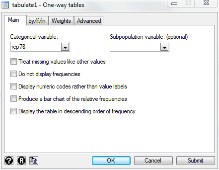
The resulting command is:
tab rep78
Note that the missing values of rep78 were not included in the table. If you want to see how many missing values you have, you should check Treat missing values like other values. Then they'll get their own entry.
Two-way Tables
Two-way tables tell you how many times each combination of two variables appears in your data. To create a two-way table, click Statistics, Summaries, tables, and tests, Tables and then Two-way tables with measures of association. Select or type rep78 for the Row variable and foreign for the Column variable, then click Submit.
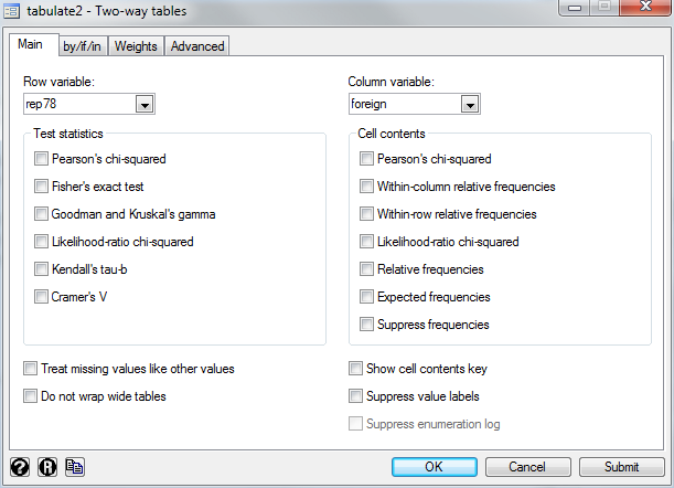
The command is:
tab rep78 foreign
Note that missing values do not appear in the table unless you check Treat missing values like other values, just like with one-way tables.
The Test Statistics section contains a variety of statistical tests which examine whether the two variables are related or not. The most commonly used is Pearson's chi-squared, better known as "the" chi-squared test. Simply check its box to have Stata run a chi-squared test on your table.
The Cell tables section allows you to add additional information to each cell of the table. The most popular are the various relative frequencies, which calculate percentages. For this table, Within-row relative frequencies answer the question "What percentage of the cars with a rep78 of one are domestic?" while Within-column relative frequencies answer "What percentage of the domestic cars have a rep78 of one?" and Relative frequencies answer "What percentage of all the cars are both domestic and have a rep78 of one?"
Correlations
To calculate the correlation between variables, click Statistics, then Summaries, tables, and tests, then Summary and descriptive statistics and finally Correlations and covariances. Then type the names of the variables you want the correlations for in the Variables box. This data set has several variables relating of the size of the cars: weight, length and displacement (a measure of the size of the engine). We would expect them to be highly correlated, but type all three in the Variables box and click Submit to verify that hypothesis.
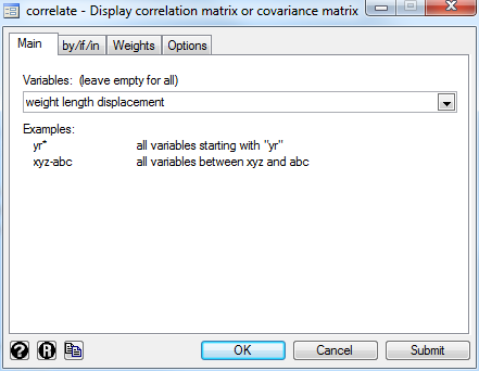
The command is:
correlate weight length displacement
Hypothesis Tests
To use a t-test to test the hypothesis that the mean of a variable is equal to some number, click Statistics, then Summaries, tables, and tests, then Classical tests of hypotheses and finally One-sample mean-comparison test. Select or type mpg as the Variable name and then type 20 in Hypothesized mean. Click OK and Stata will test the hypothesis that the mean of mpg is 20.
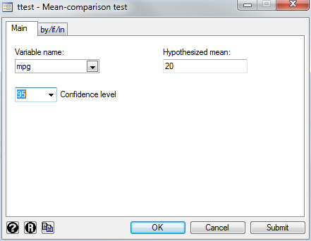
The command is:
ttest mpg==20
To test whether two variables have the same mean (assuming your data are paired), click Statistics, then Summaries, tables, and tests, then Classical tests of hypotheses and finally Mean comparison test, paired data. This test makes sense if you have two related variables (two different measures of income, for example) but since we don't have any in this data set, set First variable to weight and Second variable to price. Click OK and Stata will unsurprisingly tell you the hypothesis that their means are the same is strongly rejected.
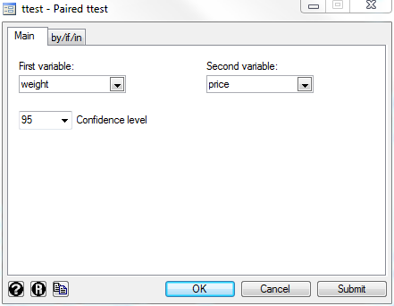
The command is:
ttest weight==price
If the data are not paired (i.e. any value of price could go with any value of weight--clearly not the case in these data the price and weight for a given observation describe the same car) you'd click on Two-sample mean-comparison test instead. This will cause Stata to use a different formula but the process of setting it up is the same.
Finally, to test whether two groups have the same mean of a single variable, click Statistics, then Summaries, tables, and tests, then Classical tests of hypotheses and finally Two-group mean-comparison test. Type or select mpg in Variable name and foreign in Group variable name, click OK, and Stata will test the hypothesis that the domestic cars and the foreign cars have the same mean mpg.
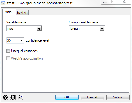
The command is:
ttest mpg, by(foreign)
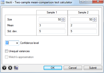
In carrying out all these tests Stata first calculates the means, standard deviations and sample sizes from your data and then plugs them into the textbook t-test formula. However, if you know those values you can put them in yourself without needing to have the actual data. click Statistics, then Summaries, tables, and tests, then Classical tests of hypotheses and finally Two-sample mean-comparison calculator. This will give you a box where you can enter the sample Size, Mean and Std. dev. for each group and Stata will carry out a t-test on the hypothesis that their means are equal.
Regression
If your class does not cover regression--or hasn't covered it yet--feel free to skip this section.
To run a basic linear regression, click Statistics, Linear models and related, Linear regression. Then type or choose mpg as your Dependent variable and type weight price foreign in Independent variables.
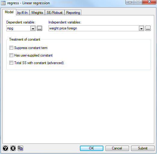
The command is:
regress mpg weight price foreign
This will regress mpg on weight, price and foreign and give you the results.
To run a logistic regression, click Statistics, Binary outcomes, Logistic regression (reporting odds ratios). (Logistic regression by itself reports coefficients, which you may also find useful). You'll then need to pick a Dependent variable and Independent variables just like with linear regression, but this time the dependent variable must be binary (1 or 0). Since foreign is the only binary variable in this data set, make it the dependent variable and make mpg weight and price independent variables.
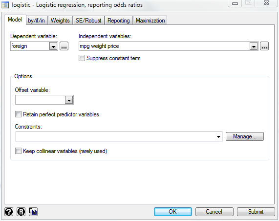
The command is:
logistic foreign mpg weight price
Stata will detect some regression problems and fix them for you automatically, such as the "dummy variable trap." But there are many, many situations where Stata will happily run a regression that makes no sense whatsoever. This example is one of them: it acts as if engineers first design a car and then decide in which country it should be built based on its characteristics. It's up to you to make sure that your regression results are meaningful.
Graphs
If your class does not require you to make graphs feel free to skip this section.
Stata has a powerful set of tools for making publication-quality graphics, but it also makes it very easy to make basic graphs.
Histograms
To make a histogram, click Graphics, Histogram then select or type mpg as the Variable. The mpg variable is continuous (in theory anyway) so leave Data are continuous selected. Under Y axis select Frequency to have the bar heights labeled in terms of number of observations in each bin. Click to Submit to see the results.
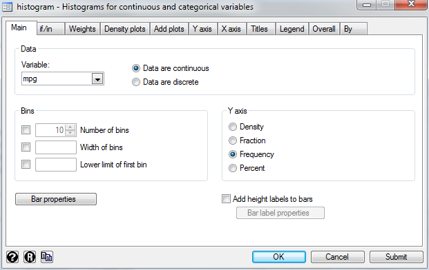
The command is:
hist mpg, freq
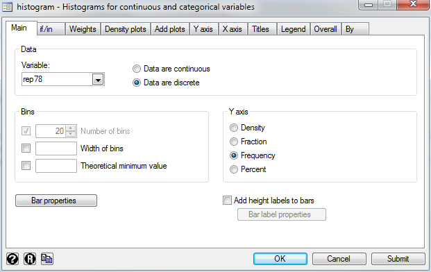
You can choose either the number of bins or the width of each bin (one implies the other). Check the box by Number of bins, type in 20 and click Submit again to see the difference it makes.
If you tell Stata that your variable is discrete the resulting histogram will have one bin for each unique value of the variable. Change Variable to rep78, choose Data are discrete and click Submit. Note that that the checkboxes under Bins are grayed out.
Scatterplots
To make a scatterplot, click Graphics, Twoway graph. By "twoway graph" Stata means just about any graph with X and Y values. The resulting window controls the "graph" meaning the entire picture you'll get. That graph can contain multiple "plots" such as scatterplots. To define a plot, click Create.
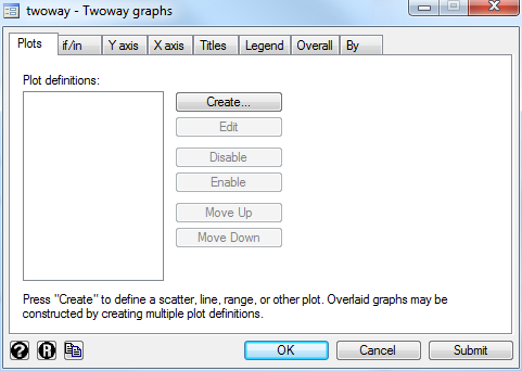
You'll then get a window for controlling that plot. Leave the plot category set to Basic plots and the type set to Scatter (but note how many other options there are). Select or type mpg as the Y variable and weight as the X variable, then click Accept. Click Ok or Submit in the main twoway window to see the graph, but note that you could also add other plots which would be overlaid on this one.
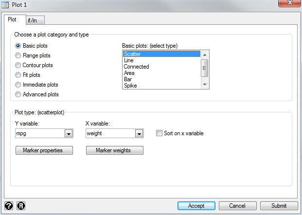
The command is:
twoway (scatter mpg weight)
or simply:
scatter mpg weight
Box Plots
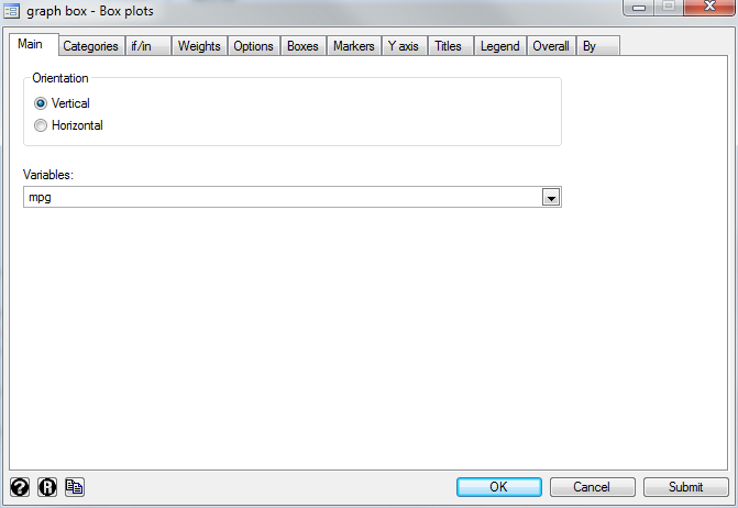
To make a Box plot, click Graph, Box and type or select mpg in Variables.
Next click on the Categories tab. Check the box for Group 1, and set the Grouping Variable to foreign. Then click OK or Submit to see the graph.
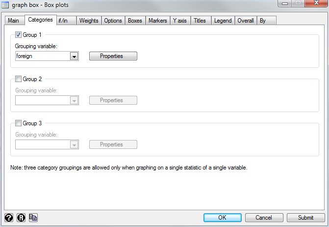
The command is:
graph box mpg, over(foreign)
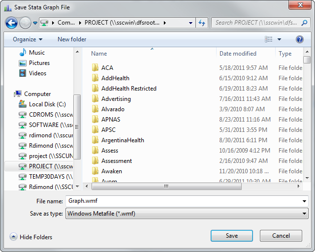
Saving Graphs
Once you've created a graph, you can save it by clicking File, Save As in the graph's window. However, note that the Stata graph format (.gph) can only be read by Stata. If you plan to use your graph in a Word document, we suggest you save it in Enhanced Metafile format (.emf). To do so, click File, Save As, and then set Save as type (near the bottom of the window) to Enchanced Metafile (*.emf). You can then insert the graph into a Word document as a picture.
Last Revised: 11/30/2011