 Supporting Statistical Analysis for Research
3.3 Relationships between continuous and categorical variables
3.3.1 Data concepts
3.3.1.1 Categorical variable
A categorical variable can take on a finite set of values.
The simplest form of categorical variable is an indicator variable
that has only two values.
The two values are typically 0 and 1, although other values are
used at times.
Other categorical variables take on multiple values.
These values are often expressed using descriptive character strings.
For example, a categorical variable for rank of a professor might
use assistant professor, associate professor, and professor
as its values.
The values of a categorical variable are sometime referred to as
levels.
Observations within a category may be more similar to other
observations within the same category and have larger
differences with observations in different categories.
These relationships are sometime referred to as within group and
between groups variation.
For example, we would expect the salaries of the assistant professor group
to be fairly similar, and to generally be different from the salaries in
the professor group.
These are the kind of relations that can be explored with graphs.
3.3.2 Exploring - Box plots
A box plot is a graph of the distribution of a continuous variable. The graph is based on the quartiles of the variables. The quartiles divide a set of ordered values into four groups with the same number of observations. The smallest values are in the first quartile and the largest values in the fourth quartiles.
The plot uses a box to show the values that are larger than the first quartile and smaller than the fourth quartile. These are the values that are closest to the center (median) of the values. The values within the first and fourth quartiles are shown as a line. These lines are referred to as whiskers. These are the values that are farthest from the center of the values.
One useful way to explore the relationship between a continuous and a categorical variable is with a set of side by side box plots, one for each of the categories. Similarities and differences between the category levels can be seen in the length and position of the boxes and whiskers.
3.3.3 Examples - R
These examples use the auto.csv data set.
We begin by using similar code as in the prior section to load the tidyverse and import the csv file.
library(tidyverse)A categorical variable is needed for these examples. The
col_typesparameter ofread_csv()is used to create a factor variable, what R calls a categorical variable. Factor variables in R will be covered in a future chapter. For now you do not need to know any more than we now can use theoriginvariable as a categorical variable.auto_path <- file.path("..", "datasets", "auto.csv") auto <- read_csv(auto_path, col_types = cols(origin = col_factor(NULL)))Warning: Missing column names filled in: 'X1' [1]glimpse(auto)Observations: 392 Variables: 10 $ X1 <dbl> 1, 2, 3, 4, 5, 6, 7, 8, 9, 10, 11, 12, 13, 14, 15... $ mpg <dbl> 18, 15, 18, 16, 17, 15, 14, 14, 14, 15, 15, 14, 1... $ cylinders <dbl> 8, 8, 8, 8, 8, 8, 8, 8, 8, 8, 8, 8, 8, 8, 4, 6, 6... $ displacement <dbl> 307, 350, 318, 304, 302, 429, 454, 440, 455, 390,... $ horsepower <dbl> 130, 165, 150, 150, 140, 198, 220, 215, 225, 190,... $ weight <dbl> 3504, 3693, 3436, 3433, 3449, 4341, 4354, 4312, 4... $ acceleration <dbl> 12.0, 11.5, 11.0, 12.0, 10.5, 10.0, 9.0, 8.5, 10.... $ year <dbl> 70, 70, 70, 70, 70, 70, 70, 70, 70, 70, 70, 70, 7... $ origin <fct> 1, 1, 1, 1, 1, 1, 1, 1, 1, 1, 1, 1, 1, 1, 3, 1, 1... $ name <chr> "chevrolet chevelle malibu", "buick skylark 320",...
3.3.3.1 Exploring - Box plots
This example uses
originas the horizontal variable for a boxplot. This results in the creation of a separate boxplot for each level of theoriginvariable. All the observation with a value of 1 are used in the leftmost boxplot. Similarly the observations for levels 2 and 3 oforiginare used in separate boxplots.ggplot(data=auto, mapping = aes(x = origin, y = mpg)) + geom_boxplot() + theme_bw()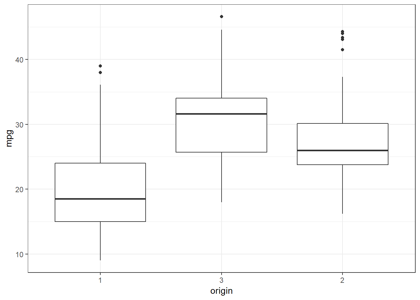
The above box plot shows that the distribution of
mpgvalues is different within the three levels oforigin. The automobiles at level 1 have a lower median value than the other two levels. The lowestmpgfor level 3 is about the median of level 1.
3.3.4 Examples - Python
These examples use the auto.csv data set.
We begin by using similar code as in the prior section to load the packages and import the csv file.
from pathlib import Path
import pandas as pd
import plotnine as p9
A categorical variable is needed for these examples. The
dtypeparameter ofread_csv()is used to create a category variable, what pandas calls a categorical variable. category variables will be covered in a future chapter. For now you do not need to know any more than we now can use theoriginvariable as a categorical variable.auto_path = Path('..') / 'datasets' / 'Auto.csv' auto = pd.read_csv(auto_path, dtype={'origin': 'category'}) print(auto.dtypes)Unnamed: 0 int64 mpg float64 cylinders int64 displacement float64 horsepower int64 weight int64 acceleration float64 year int64 origin category name object dtype: object
3.3.4.1 Exploring - Box plots
This example uses
originas the horizontal variable for a boxplot. This results in the creation of a separate boxplot for each level of theoriginvariable. All the observation with a value of 1 are used in the left most boxplot. Similarly the observations for levels 2 and 3 oforiginare used in separate boxplots.print( p9.ggplot(auto, p9.aes(x='origin', y='mpg')) + p9.geom_boxplot() + p9.theme_bw())<ggplot: (-9223371893262612655)>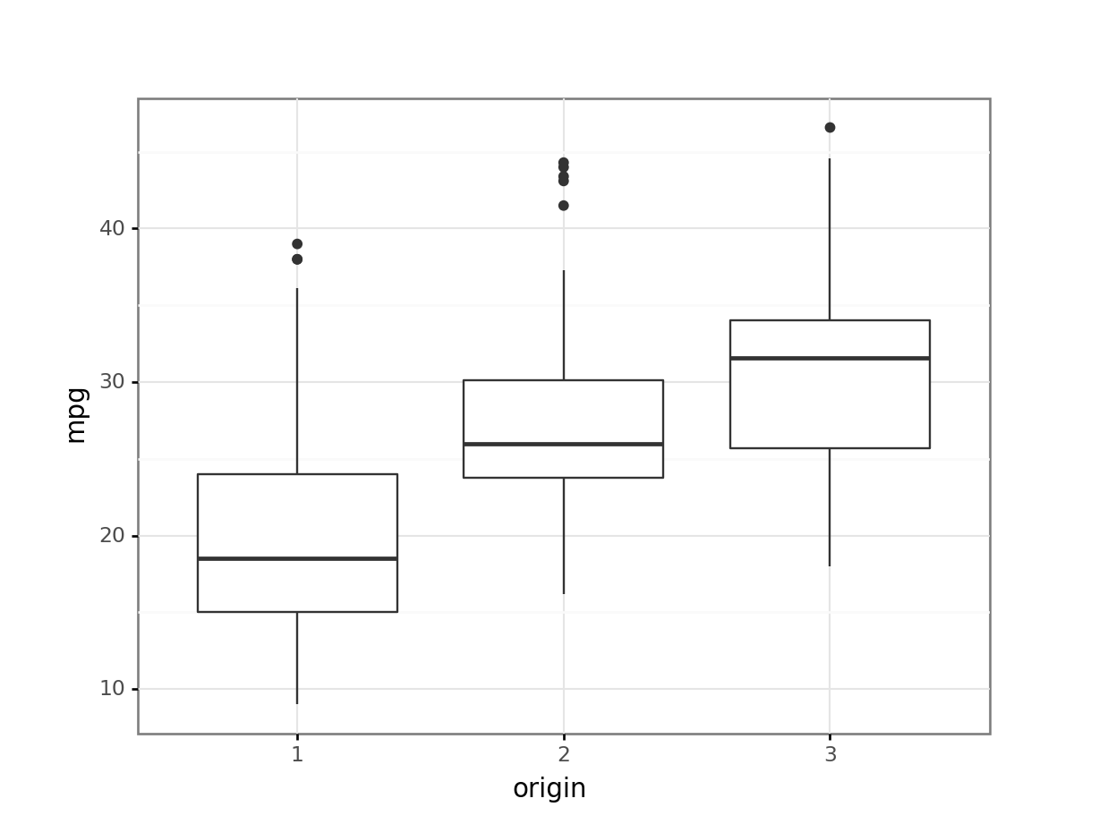
The above box plot shows that the distribution of
mpgvalues is different within the three levels oforigin. The automobiles at level 1 have a lower median value than the other two levels. The lowestmpgfor level 3 is about the median of level 1.
3.3.5 Exercises
These exercises use the Mroz.csv data set
that was imported in the prior section.
Create a boxplot for
lwgfor women who attended college and women who did not.Create a boxplot for
lwgfor men who attended college and men who did not.