SAS remains a popular and powerful tool for data management and statistical analysis. While other tools, particularly Stata, have similar capabilities and are easier to learn, most SAS experts have seen little reason to switch.
SAS is a huge program. Many of its capabilities (including those the SAS Institute seems to be most excited about) are geared towards the corporate environment rather than academia. But it would be impossible to cover even the most useful features in a single article. This article will focus on the data step, where you will be writing your own code. After reading this article you should be able to begin writing SAS programs to prepare your data for analysis right away, assuming they are in SAS format.
Using this Article
This article is based on the hands-on SAS class taught by the SSCC. Thus it is best read while sitting at the computer, actually doing the tasks described. This article is focused on SAS for Linux, so to follow the instructions exactly you will need to log in to Linstat.
You will also need to use a text editor. Any text editor will do, so if you have a favorite just make sure you can run it and save the results to the Linux file system. If you don't have a favorite, we suggest using Emacs if you are comfortable with Linux, and TextPad if you are more comfortable with Windows.
TextPad is a Windows-based editor similar to Notepad (but much better). If you are in the Social Science building and don't have TextPad on your PC, please contact the SSCC Help Desk to have it installed. To save the programs you write to the Linux file system, you will need to be logged in to the PRIMO domain. If you are working remotely the easiest way to do this is to log in to Winstat. Your Linux home directory will then be mapped as the Z: drive.
We will repeatedly be switching back and forth between the Linux shell and a text editor. You can always tell when you are supposed to type something into Linux because the text will include the prompt (the >) even though you should not type it.
You will use a fair number of small files in the course of this article. The following Linux commands will copy all of them to a directory called sasclass under your Linux home directory. Type them at the Linux prompt and hit enter after each line.
> mkdir ~/sasclass
> cd ~/sasclass
> cp /usr/global/web/sscc/pubs/files/4-18/* .
This will also make sasclass the current working directory, so you'll be all set to run the examples.
Note that SAS for Windows is the same language, and all the SAS code in this article will work in SAS for Windows. However, the process of running SAS is fairly different.
Running SAS
Servers
The SSCC has SAS installed on Winstat and Linstat. This article will focus on SAS for Linux as run on Linstat, but again, SAS syntax is the same on both Windows and Linux.
Running Programs
Linux SAS does have an interactive mode, but almost all Linux SAS users prefer to use batch mode. To run SAS in batch mode, you start by writing your program using your text editor. Once your program is written, you will give the command to run it in Linux. It will run quietly without displaying anything on the screen. However when it has finished you will find at least one and probably two new files. One is a log file, containing a record of what SAS did. This includes any error messages, so you should always look at the log after running a SAS program. If the program produced any output, it will be saved in a lst file. Both of these are text files and can be read using the same text editor you used to write the program. They can also be viewed immediately using the more command in Linux.
Normally your program should have the extension .sas (e.g. program.sas) so it is easily recognized as a SAS program (including by SAS itself). SAS will give the log and lst files the same name (e.g. program.log and program.lst).
SAS has its own special format for data sets, which cannot be read by other programs. Fortunately Stat/Transfer makes it easy to convert data sets from one format to another. Stat/Transfer is found on the Winstat servers and on Linux and is very easy to use (see Using Stat/Transfer for more information). SAS saves data sets with the extension .sas7bdat (the format has not changed since SAS 7).
Your First SAS Program
There's no substitute for actually running a SAS program if you want to see how it works. We'll begin by simply viewing the tables of an existing data set.
Data Steps and Proc Steps
SAS programs are made up of distinct steps, and each one is completed before it moves on to the next one. Data steps are written by you. They are primarily used for data manipulation (hence the name) though in theory you could do some sorts of analysis with them. Proc steps are pre-written programs made available as part of SAS. The code may look similar to a data step in some ways, but the code in a proc step is not giving SAS step-by-step instructions to execute. All you are really doing is controlling how the proc step runs. We will use a few simple procs in the course of this article, but for more details see the SAS documentation.
A step starts with either the word data or the word proc, and ends with the word run;. The run; is often not strictly required, as SAS will assume you want to start a new step when it sees data or proc. However your code will be clearer and easier to understand if you make the end of each step explicit. That may not seem very important the first time you work on a particular program, but when you have to come back to it months later and figure out what you did, you'll quickly see that saving a few keystrokes is far less important than writing clear code. Obviously if you will be sharing this code with anyone else then making it easy to understand is even more important.
Writing Your Program with a Text Editor
The time has come to actually write your first SAS program. If you want to use emacs, type
> emacs example1.sas
If you want to use Textpad, start it and immediately save the empty document as Z:\sasclass\example1.sas. This will save it in your sasclass directory on the Linux system.
As you proceed, you'll notice that both Textpad and emacs will put different words in different colors. Because the file is saved with the .sas extension, it knows you are writing SAS code and tries to make it clearer by putting official SAS commands and such in various colors. This can help you avoid mistakes.
Proc Print
Proc print simply prints the tables of a data set to the lst file. The basic syntax is
proc print data=dataset;
run;
All you have to do is specify the data set.
By default SAS will format the output such that it will be centered on a printed page. You can override this behavior by adding
options nocenter;
right before the proc print. This can make it easier to read on the screen. You can also set the line size and page size SAS will use. For example, the following will make your output fit nicely if printed in landscape mode on the SSCC's public printers:
options linesize=122 pagesize=47;
Using Data Sets
SAS uses two different types of data sets: temporary and permanent. Temporary data sets disappear when the program is completed. Permanent data sets are written as files on the disk and can be used in later programs (of course they can be deleted like any other file despite the name). To refer to a temporary data set, you simply give its name. To refer to a permanent data set, put the name and optionally the path in single quotes. If you don't specify a path, SAS will look for the data set in your current working directory.
You want to print the tables of ex1.sas7bdat, a permanent SAS data set and one of the files you copied earlier. SAS will assume the .sas7bdat extension, so all you need is:
proc print data='ex1';
run;
Type this in your text editor, and then save the file.
|
Note that proc print data='ex1'; and proc print data=ex1; Will print completely different data! |
There is an alternative way to reference a permanent data set. It used to be the only way, and many people who learned SAS before the ability to just use quotes was added never switched. The first step is to associate a SAS "library" with a directory on the disk using the libname statement:
libname library 'directory';
This command is not part of a proc or data step (it's actually what's called a global option). You can then refer to a SAS data set in that directory as library.file. For example:
libname mydata '/home/r/rdimond/sasclass';
proc print data=mydata.ex1;
run;
There are a few advanced features that only work in the context of a library, and using one could save you some typing if you repeatedly use data sets in a directory other than the current working directory. But to be honest the main reason for knowing about libraries is so you can read other people's code.
Running Your Program
Now that the program is written, you need to run it and view the results. Switch to Linux and type
> sas example1
You'll know it is done when the next prompt appears. If all went well there will now be two new files in your sasclass directory: example1.log and example1.lst. If example1.lst is missing, it's because there was an error that kept proc print from working--the log will tell you what.
A quick and easy way to view these files is with the more command. Just type
> more example1.log
and
> more example1.lst
The disadvantage is the you can't easily scroll back to view text that has already passed by. Thus the better method is to open both files in your text editor.
You should see a tremendously boring data set. If you don't, look at the log to find the error messages, and then examine your program to see what needs to be fixed.
Running your Program in the Background
This job runs so quickly it doesn't really matter how you run it, but if you have a larger job to run you may want to put it in the background. This means you'll be able to use your shell to do other work while SAS does its thing. To do this, just add an ampersand (&) to the end of the command:
> sas example1 &
You'll see a message like
[1] Done sas example1
when it is done. You can then view the output as usual. One thing you shouldn't do is start another SAS job while the first one is still running. They'll just end up competing for resources and not running any faster, but they will slow down the server's performance for other users.
Data Step Basics
The basic syntax for a data step is
data output;
set input;
{do some stuff}
run;
where output is the data set where you want to store the results, input is the data set you want to start with, and you'll add various commands to make your output more interesting that your input later.
Note how each line ends with a semicolon (;). In fact SAS doesn't care about lines, but it does demand that you put a semicolon at the end of each command. Otherwise it can't tell where one command ends and the next one begins. Whenever you find that your program is not working, especially if SAS seems to have no clue what you are talking about, the first thing to look for is a missing semicolon.
Variables
You've already seen how a SAS data set is a matrix where each row is an observation and each column is a variable. SAS has two kinds of variables: numeric and character. SAS will attempt to identify the type of a variable by what you put in it. However, once a variable is created, the type cannot be changed.
You can create or change a variable just by telling SAS what to set it equal to. The general syntax is
var=expression;
where the expression can be as simple as a number (x=5;) or include a variety of functions (x=log(exp(5));). See the online SAS documentation for a complete list of available functions and how they work.
There is one special value you should be aware of: missing, stored as a period (.). Since a data set is a matrix, every observation must have some value for each variable. If there is no valid value, SAS stores missing. Any time missing appears in an expression the result will be missing.
Change your program so that it creates a new variable z which is the sum of x and y before printing the results.
data out1;
set 'ex1';
z=x+y;
run;
proc print data=out1;
run;
Note that this will store the results in a temporary data set called out1, and the proc print has been changed to print this new data set. Run this program and take a look at the results. If you've forgotten, do that by switching to Linux and typing
> sas example1
TextPad will notice that the log and output files changed and prompt you to reload them. You'll have to tell emacs to get the new versions. Once you do, you should see that z is always 11. Don't worry, we'll be creating more interesting variables soon.
Anatomy of a Data Step
Now that you've successfully written a data step, let's take a closer look at how they work. Up to this point, everything we've done has been fairly intuitive and the results have probably been pretty much what you expected. Now we're going to see some surprises. Part of that is because we're going to intentionally abuse SAS--many of the odd behaviors you'll see can be easily avoided just by not trying to do things before the set statement. But by understanding how SAS thinks you'll be able to get it to do things that are not so obvious.
Compile Phase
SAS executes a data step in two phases. Most commands are carried out in one phase or the other. A few run in both. In compile phase, SAS checks your syntax, determines all variable types, and creates the Program Data Vector. In compile phase all relevant commands are executed exactly once, and the execution does not depend in any way on your actual data. The data is not even loaded into memory. This means you cannot do something like
if x>5 then drop x;
The drop command tells SAS not to write the variable x to your output data set. But it is executed in compile phase, and at that point SAS has no idea what the values of x are.
Execute Phase
In execute phase, your data is loaded one observation at a time, the actual work is done, and the output is written to disk. Execute phase very much depends on the actual data, and can include conditional execution (ifs) and loops. But keep in mind that all this is done after compile phase is complete.
| All Compile Phase statements
are completed before Execute Phase begins, regardless of the order they're written in! |
Order of Execution
Once you reach execute phase, SAS will load one observation and execute the entire data step before loading the next observation. So suppose you have a data set with three observations and a data step with three statements. The order of execution will be:
| Observation | Statement |
|---|---|
| 1 | 1 |
| 1 | 2 |
| 1 | 3 |
| 2 | 1 |
| 2 | 2 |
| 2 | 3 |
| 3 | 1 |
| 3 | 2 |
| 3 | 3 |
The Program Data Vector
The program data vector is SAS's work space. This is where an observation is stored while it is being worked on. Think of it as a matrix, but there is one row for each variable, and each column gives information about that variable. This includes the variable type and several "flags" that tell SAS how to process that variable. Below is an example of what a PDV looks like. We will discuss what all the various items mean in time.
| Name | Type | Length | Retain? | Missing Protect? | Keep? | Value |
|---|---|---|---|---|---|---|
| x | Numeric | 8 | Yes | No | Yes | 1 |
| z | Numeric | 8 | No | No | Yes | . |
SAS creates the PDV during compile phase and sets all but the value at that time. During execute phase the only attribute that can be changed is the value--it wouldn't make sense to have x be numeric for some observations and character for others, for example.
You should also note that the PDV only has room for one observation. When observation two is loaded, SAS has no idea what is contained in observation one or observation three. This used to be one of SAS's strengths, as it required very little memory to work with even the largest data sets. But memory is plentiful now, and you'll see that it takes some work to get around this in some situations. If your plans involve lots of calculations across observations (individuals living in households, for example) you should consider learning to use proc sql (not covered in this article) or switching to Stata.
Implicit Code
A key to understanding SAS is understanding what it adds to your data steps. This implicit code is needed to make your explicit code work, but you need to make sure it is doing what you want.
Suppose you write a data step that says:
data second;
set 'first';
run;
This simply creates a temporary copy (second) of the permanent data set first. I'll describe what SAS actually does in pseudo-code:
Top of Data Step
Set each variable to missing if its Retain flag is set
to No.
Set Statement
If there are no more observations in first.sas7bdat,
go to End of Data Step
Else read an observation
End of Code
Write each variable to temporary data set second
if its Keep flag is set to Yes
Go to Top of Data Step
End of Data Step
Note the importance of the set statement. The set statement is one of the few commands that run in both compile and execute phase. In compile phase, it tells SAS to prepare a place in the PDV for all the variables in the input data set. In execute phase, it is the set command that actually loads an observation. If you put any execute-phase code before the set statement, when that code executes all the variables will either be missing or left over from the previous observation. Finally, it is the set statement that determines when the data set ends. This means that code before the set statement will be executed one last time after the final observation has been written to the output data set.
The Retain Flag
The Retain flag is used to prevent a variable from being reset to missing at the top of the data step. This makes it a vital tool for passing information from one observation to another. Note however, that information can only move forward (without using tricks that are beyond the scope of this article). With careful use of the Retain flag, it is possible to store information from observation one until observation two can use it. But observation three will still be unknown.
The Retain flag is automatically set to yes for all variables that come from the input data set. For new variables, you can set it using the retain statement.
retain x;
will set the Retain flag to yes for the variable x. You can also set an initial value:
retain x 5;
This will set the Retain flag to yes and set the value of x to 5 in compile phase before any observations are read.
To see how this all works, go back to your program and change it to the following:
data out1;
a=x;
b=x+z;
set 'ex1';
z=x+y;
run;
proc print data=out1;
run;
Save it, run it, and look at the output. You're probably in for a surprise:
Obs    a     x    b     z     y

  1    .     1    .    11    10
  2    1     2    .    11     9
  3    2     3    .    11     8
  4    3     4    .    11     7
  5    4     5    .    11     6
  6    5     6    .    11     5
  7    6     7    .    11     4
  8    7     8    .    11     3
  9    8     9    .    11     2
 10    9    10    .    11     1
At first glance, this looks crazy. But it's perfectly logical--if you think like SAS. Take a moment and try to figure it out yourself before reading further.
The variable a is set equal to x, but before the set statement. Thus the first time it executes, no observation has been loaded and x is missing. After setting a to missing, SAS proceeds to the set statement and loads the first observation, so x is 1. When the other code is complete, SAS then goes to the top of the data set. Because x came from the input data set, its Retain flag is set to yes and x stays 1. So when SAS sees a=x; for the second time, a gets 1. Only after a is set does the second observation (x=2) get loaded. This pattern continues for all the rest of the observations, so a is always one observation behind.
Next consider b. The first time through the data step, both x and z are missing, so b is missing. Then we hit the set statement and the first observation is loaded (x=1), and then z is calculated (z=11). But then we go to the top of the data step. The Retain flag for x is set to yes automatically, but z does not come from the input data set and thus its Retain flag is set to no. So when we come to b=x+z; x is still 1, but z is missing. As a result b is also set to missing (anything + missing = missing), and this continues for all observations.
Note the order in which the variables are listed: a,x,b,z,y. This is not random--it is the order in which SAS encounters the variables in the code. In compile phase, when SAS sees a=x; it realizes it will need variables a and x, and creates entries for them in the PDV. It then adds b and z when it sees b=x+z;. Occasionally it is useful to have the variables in a certain order. You can do it by controlling the order in which SAS sees them. For example, if we wanted to make the order a,b,x,y,z, you could add
retain a b x y z;
as the first line of the data step. Of course in this case that would change the results for b (how?). It's more common that it wouldn't change anything, but there are alternative commands that really won't change anything.
The Sum Operator
SAS gives you an easy shortcut for sums; the sum operator. The syntax is simply:
var+expression;
Note that there is no equals sign, which may bother you if you have a programming background (though C++ and Java both have something kind of similar). The expression will be added to the variable, almost as if you had written
var=var+expression;
But if you use the sum operator, SAS will do several things for you automatically. First, it will set the Retain flag for the variable to yes, and give it an initial value of zero.
It will also set the Missing Protect flag to yes. Normally if you add a missing value to anything the result is a missing value. But if the Missing Protect flag is set to yes, missing values are treated like zeroes. You'll have to decide if this is appropriate for your analysis or not. But without this protection, a single missing value will make the sum missing for all subsequent observations.
To see the sum operator in action, create a new file using your text editor, and save it as example2.sas:
data out2;
set 'ex1';
count1+1;
count2=count2+1;
retain count3 0;
count3=count3+1;
count4+junk;
retain count5 0;
count5=count5+junk;
run;
proc print data=out2;
run;
Run it, and you should get the following output:
Obs     x     y    count1    count2    count3    count4    junk    count5

  1     1    10       1         .         1         0        .        .
  2     2     9       2         .         2         0        .        .
  3     3     8       3         .         3         0        .        .
  4     4     7       4         .         4         0        .        .
  5     5     6       5         .         5         0        .        .
  6     6     5       6         .         6         0        .        .
  7     7     4       7         .         7         0        .        .
  8     8     3       8         .         8         0        .        .
  9     9     2       9         .         9         0        .        .
 10    10     1      10         .        10         0        .        .
We've added five new counting variables, that add up things in various ways. Let's look at each in turn.
count1 illustrates the normal sum operator. For each observation we add one to count1, so it ends up containing the observation number.
count2 looks like it should do the exact same thing. However, we did not use the sum operator. This means that the Retain flag is not set to yes, nor is the variable initialized. As a result we are adding 1 to a missing value every time, so the result is always missing.
count3 is retained and properly initialized, so in this case it does work the same as the sum operator.
count4 and count5 illustrate the effect of the Missing Protect flag. The variable junk is never set to anything, so it is always missing. Thus even though count5 is retained and initialized just like count3, when we add junk to it it becomes missing. Because count4 uses the sum operator, its Missing Protect flag is set to yes. Thus when junk is added to it, it is treated as zero, and count4 is unchanged. Thus it never changes from its initial value of zero (which is also set automatically just because count4 uses the sum operator).
The Keep Flag
The Keep flag determines whether or not a variable is written to the output data set. It is not removed from the PDV. This means you can continue to use that variable for the duration of the current data step. However if the Keep flag is set to no, that variable will not appear in your output.
The Keep flag can be set using either the keep command or the drop command.
keep x;
will set the Keep flag for x to yes, and the Keep flag for all other variables to no. x will be the only variable in your output data set.
drop y z;
will set the Keep flag for y and z to no, and leave the Keep flag for all other variables unchanged. y and z will not appear in the output data set. Note that it is just fine if drop y z; is followed by x=y+z; since y and z are still in the PDV and can still be used.
Here's a puzzle for you. Consider the following data step:
data out;
set 'ex1';
keep count1;
count1+1;
run;
Assuming count1 does not exist until it is defined here, does it make any difference at all what data set is used for input? Could we replace 'ex1' with '2000USCensus' and get the exact same results in out?
count1 is the only variable that will be written to second. Since we're assuming it is a new variable all the variables from the input data set will be gone. So the values of the variables from the input data set don't matter. However, it is the set statement that determines when the data step is finished. So out will have the same number of observations as the input data set. Presumably a data set of US census information will have a lot more observations than the ten we have in our simple little example data set, so out would in fact look very different. Incidentally, this is why example2.sas continued to load ex1 even though we didn't care about the variables it contained: we needed some observations so we could observe the behavior of the count variables.
Subsetting If
Keep and drop allow you to control what variables (columns) make it into your output data set. A subsetting if allows you to control what observations (rows) make it. The syntax is simply
if condition;
The implicit "then" is usually described as "keep this observation" and if the condition is not true then delete it. However, this is somewhat deceptive. What really happens is that if the condition is true, the data step proceeds as usual. If it is not, then SAS jumps back to the top of the data step without writing any output. However, all code before the subsetting if is still executed. Consider the following example:
data out3;
set 'ex1';
count1+1;
if x>5;
count2+1;
run;
proc print data=out3;
run;
Put this in its own file (example3.sas) and run it. The output should look like this:
Obs     x    y    count1    count2

 1      6    5       6         1
 2      7    4       7         2
 3      8    3       8         3
 4      9    2       9         4
 5     10    1      10         5
So why are count1 and count2 so different? Both are initialized to zero because they use the sum operator. Then the first observation is loaded (x=1), and count1 is increased by 1. However, because x is not greater than 5, when SAS hits the subsetting if this observation is not written to the output data set, nor is count2 increased by one. Instead SAS jumps back to the start of the data step, loading the second observation and increasing count1 by one again. This continues until the sixth observation (x=6) is loaded and count1 increased to 6. At this point x is greater than 5 and SAS proceeds through the subsetting if. Now finally count2 increases from zero to one, and for the first time the observation is written to the output data set. As the data step proceeds, count1 and count2 both continue to increase, but count1 is always five ahead.
Where
The where statement provides a more efficient method of subsetting. If you change if x>5; to where x>5; then SAS will check to see if x>5 in the next observation before it even loads it. If it is not, SAS moves on to the next observation.
Change if x>5; to where x>5; in your program and then run it again. This time count1 is the same as count2. That's because SAS didn't even load the first five observations and thus didn't increment count1.
If you need to get some information out of the observations you drop before you drop them, a subsetting if will allow you to do that. Otherwise where is usually the better method.
_N_
While we're talking about counters, SAS has one that is built in. _N_ is an internal variable that starts at one and is increased every time SAS goes back to the top of the data step. Thus it is almost the observation number. But consider what happens after the last observation is written: SAS goes back to the top of the data step and _N_ is incremented again, so now it is one greater than the number of observations. SAS stops only when it reaches the set statement and realizes there are no more variables.
Program Flow
We've already seen how a subsetting if interrupts the flow of your program, sending SAS back to the top of the data step if a condition is not met. But you can also control the flow explicitly, executing some of your code many times or not at all, depending on your data.
If
The basic syntax for if is just
if condition then statement;
The statement will be executed only if the condition is true. For example
if x=5 then y=1;
Note that the equals sign has two distinct meanings here. In the first case it is a test: is x equal to 5? In the second case it is a command: make y equal to 1. Make sure you know which one you mean to use. There are several other logical operators:
| Symbol | Meaning |
|---|---|
| = | equal |
| ^= or ~= | not equal |
| > | greater than |
| < | less than |
| & | logical AND |
| | or ! | logical OR |
If you're used to other languages, note that != cannot be used for not equals. The logical AND and OR connect two conditions. Logical AND means the result is true only if both conditions are true; logical OR means the result is true if either condition is true. For example, suppose x=5 and y=3.
if x=5 & y=2
will be false--the first condition is true but not the second.
if x=5 | y=2
will be true.
Often logical OR is used to see if a variable takes on one of several values, but SAS has an easier alternative:
if x in(1,3,5)
will be true if x is 1, 3, or 5. You could do the same thing with
if x=1 | x=3 | x=5
but this is longer to type and harder to read.
Else
An else tells SAS what to do if the condition is not true. The syntax is:
if condition then statement1;
else statement2;
If the condition is true, then statement1 will execute. If it is not, statement2 will execute. Note that statement2 can also include an if, which allows you to deal with many possibilities. For example,
if x>0 then positive=1;
else if x<0 then negative=1;
else zero=1;
Here positive, negative, and zero are indicator variables, which will contain a one if x is respectively positive, negative, or zero.
Do Groups
But what if you want to do more than one thing if a condition is true? Fortunately you don't have to write the same if over and over. Instead you can group statements such that SAS will treat them like one. A do group begins with do; and ends with end;.
if x>5 then do;
y=3;
z=1;
end;
Note the indentation: SAS doesn't care but it will make it much easier for you to figure out what is going on.
Do Loops
Do loops (for loops in most other languages) actually have very little to do with do groups, other than using one. They are an easy way to do something a certain number of times. The syntax is
do var=i
to j;
{do stuff}
end;
var is just a utility variable called a loop counter. It keeps track of how many times you've done the loop. Normally it has no use whatsoever once the loop is done, but remember to drop it unless you really want it to be in the output data set. i and j are integers, with i<j if you want the loop to actually do anything.
When SAS first encounters your do loop, it sets the loop counter to i. It then executes commands until it hits the corresponding end;. When it sees that, it increases the loop counter by one. If at that point the counter is greater than j, it proceeds. If not, it goes back to the do statement.
Try the following (example4.sas):
data out4;
do i=1 to 10;
x=i;
end;
run;
proc print data=out4;
run;
Note that there is no input data set, and no set statement. That means the code is executed just once, except for what's in the loop. That also means just one observation is written to the output. But why is i different from x?
Obs     i     x
 1     11    10
Recall that the loop counter is incremented at the end of the loop, and then SAS decides whether to go back or not. So when i was 10, SAS repeated the loop, and set x to 10. Then i was increased to 11, SAS realized the loop was done, and it proceeded to the end of the data step. That's when the current values of x and i were written to the output.
Output
Normally SAS inserts an implicit command at the end of the data step to write the current tables of the PDV to the output data set. However, you can take control of this process with the output command. The output command tells SAS to write the PDV to the output data set immediately. Furthermore, if you include an explicit output command, SAS will not add an implicit one to the end of the data step. This allows you to write an observation more than once, or not at all.
As an example, add an output statement inside the do loop of your last program (example5.sas):
data out5;
do i=1 to 10;
x=i;
output;
end;
run;
proc print data=out5;
run;
We now have ten separate observations. Furthermore, the final value of i changed. Why?
Obs     i     x

  1     1     1
  2     2     2
  3     3     3
  4     4     4
  5     5     5
  6     6     6
  7     7     7
  8     8     8
  9     9     9
 10    10    10
Previously, when i was set to 11 the do loop ended, SAS reached the end of the data step, and the observation was written. Now that you have included an explicit output statement, the implicit output at the end of the data step is removed. i is still set to 11, but we never see it because it only happens after the last output statement.
Arrays
One of the most common uses for do loops is to do the same thing to many variables. However, to do this we need a way to refer to a collection of variables by number. SAS does this by defining arrays. An array in SAS is different from any other programming language. It is not used to store information; it is not a variable. Rather, it is another way of referring to existing variables--a way that is highly convenient for do loops.
To define an array, the syntax is
array name(n) variable1 variable2...;
For example:
array vars(3) x y z;
Once we've done this, vars(1) is just another name for x, vars(2) for y and vars(3) for z.
Let's double the values of all the variables in our data set (example6.sas).
proc print data='ex1';
run;
data out6;
set 'ex1';
array vars(2) x y;
do i=1 to 2;
vars(i)=vars(i)*2;
end;
run;
proc print data=out6;
run;
Now in this case setting up the array and the do loop was a good bit more work than just writing
x=x*2;
y=y*2;
But suppose you had a hundred variables--then the advantage would be obvious.
Note that array definitions only last for the duration of the data step. But they are easy to copy and paste from one data step to another.
Variable Lists
On the other hand, writing out the names of all one hundred variables would get pretty tedious. Fortunately SAS has some shortcuts for writing out lists of variables. They can be used in more than just array definitions (you can use them in retain, drop, and keep statements for example), but they are particularly useful in array definitions.
If you have variables with some sort of stem and then a number (var1, var2, var3, etc.) you can use a number list. Just put a dash between the first and last variables (var1-var3).
You can always use a position list. Suppose you had variables a, b, c, x, y, z, in that order. You could refer to them all by putting a double dash between a and z (a--z). Just remember that the variables must be in the proper order for this to work--recall our discussion of how SAS decides what order to put variables in.
There are also several special purpose lists you can designate by name. These include _all_ for all variables, _numeric_ for all numeric variables, and _character_ for all character variables.
Finally you can use a wildcard. The colon (:) will match anything, or nothing. For example, var: would include var, var1, var2, variable, variety, and anything else that starts with var.
These kinds of shortcuts can sometimes make it less than obvious just how many elements your array has. In your array definition you can just put an asterisk (*) in the parenthesis and SAS will give the array as many elements as there are variables in your list. You can also use the dim() function to find out how many elements an array has, for example to figure out how many times a do loop needs to execute. Try the following changes (example7.sas--just save example6.sas with the new file name and then make the changes):
proc print data='ex1';
run;
data out7;
set 'ex1';
array vars(*) _all_;
do i=1 to dim(vars);
vars(i)=vars(i)*2;
end;
run;
proc print data=out7;
run;
Note that i was not doubled. Why?
Obs     x     y    i

  1     2    20    3
  2     4    18    3
  3     6    16    3
  4     8    14    3
  5    10    12    3
  6    12    10    3
  7    14     8    3
  8    16     6    3
  9    18     4    3
 10    20     2    3
Remember that SAS works through the code line by line in compile phase. So when it saw the array definition, it had not yet seen any reference to the variable i. Thus i was not yet in the PDV, and _all_ consisted solely of x and y. This can be a good thing--it can be really confusing if you're trying to loop over an array that contains the loop counter.
A puzzle for you: if i had been defined before the array (say, with a retain statement), what value would it have in the output data set?
The answer is 7. Can you see why?
By, First, and Last
Often data sets have some sort of group structure. For example, individuals may live in households. To be honest, SAS data steps don't handle this kind of situation very well, because they only have one observation in memory at a time. If you are planning to work with this kind of data, you should consider learning either proc sql or Stata. But the tools SAS does have are important to learn.
The first step is to identify what makes up a group. You do this with the by statement. The syntax is just:
by variable1 variable2...;
For example, if hhid was a household id,
by hhid;
This allows you to use first and last. These are conditions that will be true if SAS currently has the first or last observation of the group in memory. The syntax is first.variable or last.variable, as in
if first.hhid then (do something);
else if last.hhid then (do something else);
There is one additional requirement for using by, and that is the data must be sorted by the by variables. Which leads us to...
Proc Sort
Proc sort is a utility proc that sorts data. The syntax is
proc sort data=input out=output;
by variables;
run;
where input is an existing data set and output is a data set that will be created. For example,
proc sort data=first out=second;
by x;
run;
If you list more than one variable, the data set will first be sorted by the first variable in the list, then ties will be sorted by the second variable, etc. If you need to sort in descending order, just add the word descending before that variable. For example:
proc sort data=first out=second;
by x descending y;
run;
Example: Working with Households
We're now going to do an example. As we work through it, try to think of your own solutions, but don't be discouraged if you nothing workable comes to mind. Learning to think like SAS is important but it takes time. As you'll see later there's an easier way to do this task using a proc, but it's important to know how to do such things yourself for those times when you need to calculate something that isn't built into a proc.
Start by taking a look at the tables of ex2.sas7bdat. You should have no problem writing a program that will allow you to do so, so try before you read on.
The solution, of course, is just a proc print:
proc print data='ex2';
run;
We have here a data set of individuals, each living in households. You are given the income of each individual, but your task is to create a new variable containing the total household income of each household. Before proceeding, try to describe how to do this in English. The trick is to remember that SAS only knows about one observation at a time.
The basic procedure will be to add up the income from each individual. But this means the calculation won't be complete until we reach the last individual in each household. So the second step will be to reverse the order of the observations and then take that correct value of household income from the last observation and copy it to all the other observations (remember information can only move forwards).
As a first try at the first part, try the following.
data step1;
set 'ex2';
hhinc+income;
run;
proc print data=step1;
run;
What is wrong? What's needed to fix it?
Obs    hhid    id    income     hhinc

  1      1      1     30000     30000
  2      1      2     45000     75000
  3      1      3         0     75000
  4      2      4     60000    135000
  5      2      5     55000    190000
  6      3      6     42000    232000
  7      4      7     90000    322000
  8      4      8     15000    337000
  9      4      9         0    337000
 10      5     10     25000    362000
The problem is that the hhinc variable is ending up with a running sum of all incomes, not just the incomes of the people in each household. What we need is a way to "start over" when we start a new household. Try to write it before reading the following:
data step1;
set 'ex2';
by hhid;
if first.hhid then hhinc=0;
hhinc+income;
run;
proc print data=step1;
run;
The output will be:
Obs    hhid    id    income     hhinc

  1      1      1     30000     30000
  2      1      2     45000     75000
  3      1      3         0     75000
  4      2      4     60000     60000
  5      2      5     55000    115000
  6      3      6     42000     42000
  7      4      7     90000     90000
  8      4      8     15000    105000
  9      4      9         0    105000
 10      5     10     25000     25000
So now you have the correct household income, but only for the last individual in the household (actually, the last person with a non-zero income and everyone after them). Now you need to make that last observation first. Obviously this will require proc sort, but try to write it yourself.
proc sort data=step1 out=step2;
by hhid descending hhinc;
run;
This sort doesn't necessarily reverse the order of observations in each household, but it does guarantee that someone with the correct household income will be first in each household. Now you just need to give every person in each household the same value for household income as the first person in that household. The easiest way involves creating a new variable and then dropping our current hhinc. See if you can take it from there before proceeding.
data final;
set step2;
by hhid;
retain hhincome;
if first.hhid then hhincome=hhinc;
drop hhinc;
run;
proc print data=final;
run;
Note that hhincome is retained. This means it is only changed when we explicitly change it. When we reach the first observation in a new household, we set hhincome to their hhinc variable (recall that this value is correct for the first observation in each household). For the second and subsequent observations, hhincome simply stays the same. Add a proc print so you can see the results and you're done.
Obs    hhid    id    income    hhincome

  1      1      2     45000      75000
  2      1      3         0      75000
  3      1      1     30000      75000
  4      2      5     55000     115000
  5      2      4     60000     115000
  6      3      6     42000      42000
  7      4      8     15000     105000
  8      4      9         0     105000
  9      4      7     90000     105000
 10      5     10     25000      25000
For an alternative way of doing the same task, see the example under merging.
Example: Reshaping Data
Any data that has groups and subgroups (for example, individuals living in households) can be presented in two forms. In the long form, each subgroup has its own observation--the data set used in the last example was in this form. In the wide form, each group is just one observation, and there is a separate set of variables for each subgroup. The dataset whh.sas7bdat is in this form. For whatever reason the wide form seems to be more common with data sources. However, the long form is usually more useful for analysis. So it is a common task to have to reshape data from the wide form to the long. We'll also learn how to convert long to wide, just in case.
In the long form you will have just one age and one sex variable for each individual, not the four age and sex variables per observation you have now (note that sex is stored as an indicator variable). You will also be creating multiple observations from each currently existing observation. This calls for putting an output statement inside a do loop. Since you're using a do loop, you will have a loop counter variable telling you which observation you're writing--you can also use this to pick which age and sex to write by putting them all in an array. Consider this as a first try:
data long;
set 'ex3';
keep hhinc hhid age sex;
array ages(4) age1-age4;
array sexes(4) sex1-sex4;
do i=1 to 4;
age=ages(i);
sex=sexes(i);
output;
end;
run;
proc print data=long;
run;
Here i is your loop counter, but it also tells you which observation you're writing. When i is one, you are writing the first individual in the household, and thus set age to age1 and sex to sex1. When i is 2, we are working with the second individual and use age2 and sex2, etc. There's just one problem with the result. Can you see it?
Obs    HHID    HHINC    age    sex

  1      1     50000     30     0
  2      1     50000     28     1
  3      1     50000      3     0
  4      1     50000      .     .
  5      2     80000     45     0
  6      2     80000     47     1
  7      2     80000     12     1
  8      2     80000      8     0
  9      3     40000     25     1
 10      3     40000      .     .
 11      3     40000      .     .
 12      3     40000      .     .
Because every observation must have all variables, our original data has ages and sexes defined for four people in each household. However, they are all needed only in household two. Household one has three members, and household three has just one. But our program creates four observations per household regardless.
The solution is to add an if condition before the output statement. We will only output an observation if either sex or age is non-missing. If both variables are missing, we assume the person does not actually exist. This is not an entirely innocuous assumption. It does not distinguish between a household with less than four people and a household containing a person whose sex and age really weren't determined. However, it is usually unavoidable. In the wide form, the number of variables is determined by the largest group, so in real data sets there may be room for twenty or more individuals in each household. Leaving them all in your analysis is probably not an option.
The appropriate modification is:
data long;
set 'ex3';
keep hhinc hhid age sex;
array ages(4) age1-age4;
array sexes(4) sex1-sex4;
do i=1 to 4;
age=ages(i);
sex=sexes(i);
if age~=. | sex~=. output;
end;
run;
proc print data=long;
run;
And the result will be:
Obs    HHID    HHINC    age    sex

 1       1     50000     30     0
 2       1     50000     28     1
 3       1     50000      3     0
 4       2     80000     45     0
 5       2     80000     47     1
 6       2     80000     12     1
 7       2     80000      8     0
 8       3     40000     25     1
Now let's convert it back. This time, you need to combine multiple observations into one observation. But you won't need to write a loop: SAS is already looping over observations. What you will need to do is keep track of which observation in the household you are working with, and then write the result when you are all done. "All done" means you've read the last observation, so that's a job for by and last. Keeping track of which observation you're on is a job for a loop counter, so we'll create one for ourselves even though SAS is doing the looping. Add the following to your code.
data wide;
set long;
array ages(4) age1-age4;
array sexes(4) sex1-sex4;
by hhid;
if first.hhid then n=1;
ages(n)=age;
sexes(n)=sex;
if last.hhid then output;
n+1;
drop n sex age;
run;
proc print data=wide;
run;
Try running this. What's wrong?
Obs    HHID    HHINC    age1    age2    age3    age4    sex1    sex2    sex3    sex4

 1       1     50000      .       .       3       .       .       .       0       .
 2       2     80000      .       .       .       8       .       .       .       0
 3       3     40000     25       .       .       .       1       .       .       .
The last person in each household is being stored properly, but the others are missing. That's because the age and sex variables are not retained. Thus SAS resets them to missing every time it loads a new observation. So when we get to the last observation in each household, all the previous information is gone. The solution is just to add a retain statement:
data wide;
set long;
retain age1-age4 sex1-sex4;
array ages(4) age1-age4;
array sexes(4) sex1-sex4;
by hhid;
if first.hhid then n=1;
ages(n)=age;
sexes(n)=sex;
if last.hhid then output;
n+1;
drop n sex age;
run;
proc print data=wide;
run;
Try running it again. Now what's wrong?
Obs    HHID    HHINC    age1    age2    age3    age4    sex1    sex2    sex3    sex4

 1       1     50000     30      28       3       .       0       1       0       .
 2       2     80000     45      47      12       8       0       1       1       0
 3       3     40000     25      47      12       8       1       1       1       0
The problem is household three. It should have just one individual living in it, but our data set lists four. The other three came from household two. Retain doesn't do anything special as a result of by groups, so when we moved from household two to household three, all the age and sex variables stayed the same. age1 and sex1 were then overwritten by the actual person living in household three, but the other variables were not.
We need to tell SAS to set all the ages and sexes to missing when we are ready to move on to a new household. This is easy to do:
data wide;
set long;
retain age1-age4 sex1-sex4;
array ages(4) age1-age4;
array sexes(4) sex1-sex4;
by hhid;
if first.hhid then n=1;
ages(n)=age;
sexes(n)=sex;
if last.hhid then do;
output;
do i=1 to 4;
ages(i)=.;
sexes(i)=.;
end;
end;
n+1;
drop i n sex age;
run;
proc print data=wide;
run;
Note how the indentation makes it easy to see the logic of the program, even though we have several different layers. Your output should be:
Obs    HHID    HHINC    age1    age2    age3    age4    sex1    sex2    sex3    sex4

 1       1     50000     30      28       3       .       0       1       0       .
 2       2     80000     45      47      12       8       0       1       1       0
 3       3     40000     25       .       .       .       1       .       .       .
Data Set Options
SAS can do some work with an input data set before your data step ever sees it, or with an output data set after your data step is done with it. You control this by setting various data set options. These are statements in parenthesis immediately following the data set name--either the name of the output data set in the data statement, or the name of the input data set in the set statement. They can also be used in procs. For example:
proc print data=bigDataSet (obs=20);
run;
This will print just the first 20 observations from bigDataSet, so you can look them over.
Some of the more commonly used options include:
(obs=n)
This causes SAS to stop processing after n observations. This is extremely useful in testing your code. You can have SAS run your program on just the first 100 observations to make sure it works, or have SAS print just some of the observations so you can look at them, as in the above example.
(where=(condition))
This has the same function as the where statement. Observations which do not meet the condition are never even loaded. The differences are where it goes (right after the data set as opposed to its own line) and the equals sign.
(drop=(variables))
(keep=(variables))
These are similar to the keep and drop commands inside a data step (again note the equals sign), but if applied to the input data set the variables not selected are never loaded. Again, it as if they didn't exist.
(rename=(oldName1=newName1 oldName2=newName2))
This option allows you to rename variables, and if applied to input the name is changed before the data is even loaded.
If you want to apply more than one option, they go in the same set of parentheses:
proc print data=bigDataSet (obs=20 where=(x>10));
run;
Note that your code will be run more quickly if it has to work with less data. If you will be cutting down the number of observations or variables at some point, doing it with using data set options on the input data set where possible will be the most efficient.
Combining Data Sets
Combining data sets is a very common task in SAS. Often the data come in pieces or from multiple sources, or you may generate a data set you need to combine with the original data. SAS has a couple different tools for combining data sets, depending on how they need to go together.
Appending Data Sets
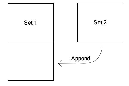
If you just need to add the observations from two data sets together, this is called appending. For example if you had one data set of domestic cars and another of foreign cars, you could append them to make a single data set of all cars. Normally you would only do this if the two data sets have the same (or almost the same) variables. If one data set has a variable that the second data set doesn't, all the observations from the second data set will be assigned missing values for that variable.
Appending data sets if very simple in SAS: simply list all the data sets you wish to append in the set statement. Consider the following:
data combined;
set set1 set2 set3;
run;
The output data set, combined, will contain all the observations from set1, then all the observations from set2, and finally all the observations from set3. It will have all the variables used by any of these data sets, and if any of the input data sets are missing a variable it will be missing in that data set's observations.
Merging
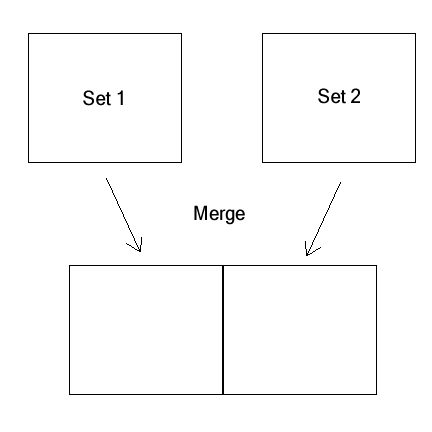
If two data sets have the same (or almost the same) observations but different variables, you combine them with a merge. For example, if one data set had car names and prices, and another had car names, weights, and fuel efficiency, you could merge them to create a singe data set with all the data available. Note that if a car appeared in one data set but not the other, it will have missing values for all the variables from the other data set.
Note that in my example, name appeared in both data sets. This is important because it will be the identifier used to link observations. Assuming every car has a unique name, this is an example of a one-to-one merge. But suppose you had one data set of individuals including the state they live in, and another data set containing welfare benefit levels for each state. You could perform a merge that creates a data set of individuals and the welfare benefits available to them, but each state would be merged with many individuals. This is an example of a one-to-many merge. Logically it is also possible to have many-to-many merges, but these are more likely to be the result of logical errors or problems with the data sets.
The syntax for a merge is the same no matter what kind it is:
data combined;
merge set1 set2;
by matchvar;
run;
Here matchvar is the variable that will be used to link the observations. In our first example, it would be the name of the car; in the second the name of the state. It is possible to link by multiple variables. In that case observations will be merged only if they have the same values for all the match variables.
Sometimes it's important to know whether an observation was successfully matched between the two data sets. For example, you may want to get rid of observations that are incomplete (be careful though, as this could bias your analysis). You can tell SAS to create a new variable indicating whether a data set contributed to an observation with the in data set option. The syntax is just in=variable, but the variable thus created is only temporary. It's gone even before you can use it in data set options for the output data set. So if you need to keep those values, store them in another variable. Here's another version of the last example, but one which only keeps observations that exist in both data sets:
data combined (drop=in1 in2 where=(in1=1 & in2=1));
merge set1 (in=temp1) set2 (in=temp2);
by matchvar;
in1=temp1;
in2=temp2;
run;
Example: Households Again
An alternative way to find household incomes is let proc means do all the hard work and then merge in the results. See the SAS documentation for more details about proc means. We will use it to create a data set containing just the household incomes for each household:
proc means data='ex2';
by hhid;
var income;
output out=households sum(income)=hhincome;
run;
proc print data=households;
run;
The households data set will contain the following:
Obs    hhid    _TYPE_    _FREQ_    hhincome

 1       1        0         3        75000
 2       2        0         2       115000
 3       3        0         1        42000
 4       4        0         3       105000
 5       5        0         1        25000
We have a couple extra variables we don't need, but we'll get rid of them later. Now all we need to do is merge the household income data with the original data set. Note that this is a one to many merge (one household matches with many individuals) and that our match variable is hhid. We'll also get rid of the extra variables proc means created.
data hhincomes;
merge 'ex2' households (drop=_TYPE_ _FREQ_);
by hhid;
run;
proc print data=hhincomes;
run;
You'll notice that this method is shorter and simpler than what you did before--which is what you would expect since you used a pre-written tool (proc means) rather than doing all the work yourself. The previous example was mostly intended as a learning experience, though if you needed to calculate a function not covered by proc means you might have to do something similar.
Using your Log File
In the unlikely event it hasn't happened already, be aware that quite often your programs won't run properly the first time. Or the second. Or the third. Debugging often takes as long as writing the program itself, or longer. In these cases your best hope for understanding what SAS thinks your program means (as opposed to what you think it means) is to look closely at your log file.
SAS puts a lot of information in your log file--sometimes too much. It can be tempting to skip looking at it and jump straight to the output (the .lst file). Resist this temptation. An error in your code can make your output meaningless. One common scenario is that the program failed before reaching the commands that generate output and as a result the .lst file you're reading is from a previous, presumably even more buggy, run. Your text editor can help you: do a search for the word ERROR. If it doesn't exist, at least you know your program ran all the way through (though you don't know for sure it did what you intended). If it does, you'll know where things went wrong.
If you do find a syntax error, some of the most common causes are simple.
Missing Semicolon
This is undoubtedly the most common error. The problem here is that SAS will attempt to interpret the next command as part of the last command. What makes it particularly confusing is that SAS will blame the error on the command after the missing semicolon, so you may miss the problem with the line above. Here's an example from some code we've used previously:
keep hhinc hhid age sex
array ages(4) age1-age4;
Note that there should be a semicolon at the end of the first line. Here is an excerpt from the log:
4          data long;
5          	set 'whh';
6          	keep hhinc hhid age sex
7          	array ages(4) age1-age4;
                     _
                     22
                     76
ERROR 22-322: Syntax error, expecting one of the following: a name, -, :, ;, _ALL_, _CHARACTER_, _CHAR_, _NUMERIC_.

ERROR 76-322: Syntax error, statement will be ignored.

8          	array sexes(4) sex1-sex4;
9          	do i=1 to 4;
10         		age=ages(i);
                 ____
                 68
ERROR 68-185: The function AGES is unknown, or cannot be accessed.
Note the line underneath the word ages(4), with two numbers underneath that. That indicates where SAS ran into a problem, and the numbers direct you to the corresponding ERROR messages. SAS still thinks it's working on a keep statement, so it's looking for variables or lists of variables. array is a perfectly good variable name (which is unfortunate in a some ways) but ages(4) fails because of the parentheses.
The second error message arises because the array ages() has not been defined. Thus SAS thinks it is a function. This is a common problem: one error causes a cascade of error messages later in the code. Normally if you can see and correct one error, it's worthwhile to run the program again before spending any significant time trying to figure out any subsequent errors. They may take care of themselves.
Endless Quotes or Comments
SAS uses quotes--single or double--to mark off text that should be treated in a special way. If the end quote is missing, SAS will get very confused. Consider the following:
set 'whh;
Note the missing single quote at the end of the file name. In the log you'd see that SAS got to this point, and then the entire rest of the program will be printed to the log without any indication SAS tried to execute it. Finally, you'll see SAS complaining that it's not seeing what it's expecting and that it can't open a data set.
The problem is that without an end quote, SAS thinks the entire rest of the program is the file name for the input data set. And since it still doesn't end with a quote and a semicolon, you finally get an error message at the end of the program.
A related problem can occur with comments. SAS will ignore any text in between /* and */. This allows you to write explanatory notes for yourself or others that read your code--a very good idea. However, if you forget the */ at the end, the rest of your program will be ignored completely.
TextPad and Emacs with ESS make it easy to catch these kinds of errors because they put strings in quotes and comments in distinctive colors. If half your program suddenly turns "comment green" that's a good indication that you forgot to end a comment somewhere in the middle of it.
Typos
Obviously any typos in your code may cause problems. It's not as guaranteed as you might think:
dat long;
will actually get you:
WARNING 14-169: Assuming the symbol DATA was misspelled as dat.
As long as SAS is correct, this is good. Obviously there are limits:
da long;
gets you:
4          da long;
           __
           180

ERROR 180-322: Statement is not valid or it is used out of proper order.

5          	set 'whh';
            ___
            180

ERROR 180-322: Statement is not valid or it is used out of proper order.

6          	keep hhinc hhid age sex;
            ____
            180


ERROR 180-322: Statement is not valid or it is used out of proper order.
Note the cascading failure again here. Because SAS doesn't realize you're starting a data step here, all the data step commands don't make sense. Change da to data, and all the rest will go away.
Once again, syntax coloring can help you here. If you're trying to type a SAS command and it doesn't turn "command blue," you know there's a problem.
You can run into more subtle problems if you mistype a variable. SAS does not have any special syntax to create a variable. It is placed in the PDV as soon as you mention it in the code. For example, if you accidentally type
keep hhinc hhid age srx;
where srx is meant to be sex, the code still runs. The only indication of trouble is a warning in the log:
WARNING: The variable srx in the DROP, KEEP, or RENAME list has never been referenced.
Then when you try to use sex later, in your second data step, you get
NOTE: Variable sex is uninitialized.
It was supposed to come from the results of the first data set, but it was dropped because it wasn't on the list of variables to keep. But a warning or a note doesn't stop your program from running. It will proceed and do what SAS thinks you intended. But the results will be nonsense. This demonstrates the importance of looking carefully at your log even if the program ran to completion and gave you the output you expected.
Learning More
You now have a good background in how data steps work, but there's much more to learn. The SSCC has a variety of articles on specific topics in SAS--take a look at our Knowledge Base.
For a broad but somewhat shallow introduction to SAS, The Little SAS Book by Delwiche and Slaughter is the standard, and is available in the CDE library. The SAS online documentation of course can tell you everything you need to know, but it can be a challenge to read.
Finally, the SSCC Help Desk will be happy to answer any questions you may have about SAS. From 1-4 every afternoon the consultant on call will be someone familiar with SAS. But you can email the Help Desk or call 262-9917 at any time and your question will be referred to the person who can best answer it.
Last Revised: 1/22/2007