A chief executive officer (CEO) is a leader of a firm or organization. The CEO leads by developing and implementing a strategic policy for the firm. The CEO is in charge of a management team that is responsible for the daily firm operations, financial strength and corporate social responsibilities.
The CEO also leads the firm in compensation. Generally, a CEO is the most highly paid person in a firm; CEO salaries are at the top of the pyramid. Although some industries have employees whose salaries exceed the CEO’s, for example sales agents, the broad rule is that CEO salaries form an effective upper bound for employee compensation. Thus, although very few managers ever become chief executive officers, there is a great deal of interest in CEO salaries. CEO compensation indirectly influences salaries for a large portion of the firm workforce.
CEO salaries in the United States are of interest because of their relationship to salaries in international firms and to salaries of people that do not belong to Corporate America. Top managers in the United States have come under a great deal of criticism for being so highly paid compared to their international counterparts. Yet, compensation of CEOs may not be out of line compared to top professionals in other fields. For example, Linden and Machan (1992, “Put Them at Risk!” Forbes Magazine, p. 158) compares CEO salaries with professionals such as actors, models, surgeons, sports personalities and so on, and finds the compensation comparable.
Measuring annual compensation for a CEO is fraught with difficulties. Compensation clearly includes salary plus bonuses, that is, cash payments that may or may not be performance related. Other compensation is more difficult to measure and may include restricted stock awards and contributions to retirement, health insurance, and other employee benefit plans. Remuneration may also come in the form of stock gains based on the CEO’s stock ownership or exercise of stock options, although we did not consider this source of income.
The data for this study were drawn from the May 25, 1992 issue of Forbes Magazine entitled “What 800 Companies Paid for their Bosses.” This article provides several measures of CEO compensation, as well as characteristics of the CEO and measures of his firm’s performance. We say “his” because of the 800 CEOs studied in this article, only one was a woman. The goal of this report is to study CEO and firm characteristics to determine the important factors influencing CEO compensation.
To understand the determinants of CEO compensation, one hundred observations were randomly selected from the 800 listed in the Forbes article. Although the Forbes article did not cite the basis for a firm to be included in its survey, the 800 companies seem to represent the largest publicly traded companies in the United States. Our sample of one hundred CEOs and their firms represent a cross-sectional sample of America’s largest corporations. In our cross-section, the CEO and firm characteristics were based on 1991 measures.
Table 1 provides variable definitions.
$$
{scriptsize
begin{matrix}{large text{Table 1. Variable Definitions} }\
begin{array}{ll} hline
Variable & Definitions \
hline
text{COMP} & text{Sum of salary, bonus and other 1991 compensation, in thousands of dollars.} \
& ~~~text{Other compensation does not include stock gains}. \
text{AGE} & text{CEOs age, in years} \
text{SALES} & text{1991 sales revenues, in millions of dollars} \
text{TENURE} & text{Number of years employed by the firm} \
text{EXPER} & text{Number of years as the firm CEO} \
text{VAL} & text{Market value of the CEOs stock, in thousands of dollars} \
text{PCTOWN} & text{Percentage of firm’s market value owned by the CEO } \
text{PROF} & text{1991 profits of the firm, before taxes, in millions of dollars} \
text{EDUCATN} & text{Education level.} \
& 0 text{ indicates that the CEO does not have an undergraduate degree} \
& 1 text{ indicates that the CEO has only an undergraduate degree} \
& 2 text{ indicates that the CEO has a graduate degree} \
text{BACKGRD} & text{Categorical variable to professional background of the CEO} \ hline \
end{array}
end{matrix}
}
$$
Part I. Preliminary Summarization.
1. From a preliminary examination of the data, the 51st observation, had an unusually low compensation. This was Craig McCaw, CEO of McCaw Cellular, who reported a salary of $155,000 in 1991. This was despite a five-year total reported salary of over fifty-three million dollars. As founder of McCaw Cellular, Mr. McCaw received a substantial amount of remuneration outside of figures reported in 1991. Omit him from the sample.
Solution
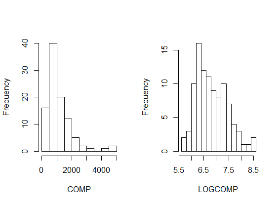
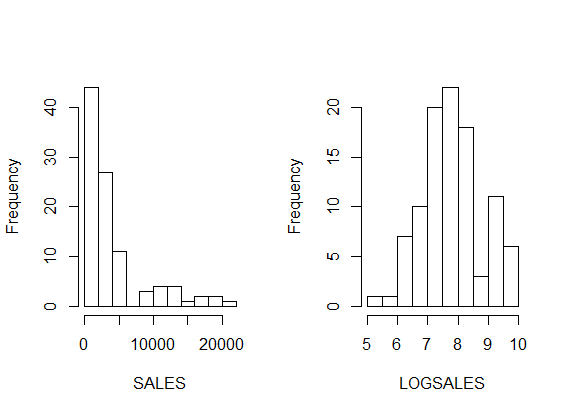
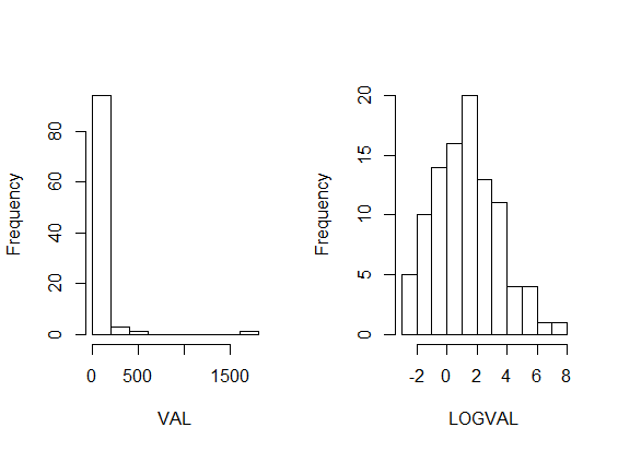
2. Create the variables LOGCOMP, the natural logarithm of COMP, LOGSALES, the natural logarithm of SALES and LOGVAL, the natural logarithm of VAL.
- 2a. Create histograms of COMP and LOGCOMP; compare the two distributions, commenting in particular on the effect that the logarithmic transformation has on the symmetry.
- 2b. Do this also for SALES and VAL.
3. Compute summary statistics of the continuous variables COMP, LOGCOMP, AGE, SALES, LOGSALES, TENURE, EXPER, VAL, LOGVAL, PCTOWN, and PROF. Identify the median value of each variable.
Solution
Part II. Basic Linear Regression.
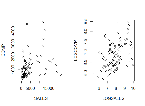
1. Plot SALES versus COMP and then LOGSALES versus LOGCOMP. Discuss the difficulties in modeling the relationship between SALES versus COMP that are not apparent in a relationship between LOGSALES and LOGCOMP.
Solution
2. Compute correlations among the continuous variables COMP, LOGCOMP, AGE, SALES, LOGSALES, TENURE, EXPER, VAL, LOGVAL, PCTOWN, and PROF. Identify the variable (excluding LOGCOMP) that seems to have the strongest relationship with COMP. Also, identify the variable (excluding COMP) that seems to have the strongest relationship with LOGCOMP.
Solution
3. Fit a basic linear model, using LOGCOMP as the outcome of interest and LOGSALES as the explanatory variable.
- 3a. Interpret the coefficient associated with LOGSALES as an elasticity.
- 3b. Provide 90% and 99% confidence intervals for your answer in 3a.
Part III. Multiple Linear Regression - I.
1. Create a binary variable, PERCENT5, that indicates whether the CEO owns more than five percent of the firm's stock. Create another binary variable, GRAD, that indicates EDUCATN=2.
Solution
2. Run a regression model using LOGCOMP as the outcome of interest and four explanatory variables, LOGSALES, GRAD, PERCENT5, and EXPER.
- 2a. Interpret the sign of the coefficient associated with GRAD. Comment also on the statistical significance of this variable.
- 2b. For this model fit, is EXPER as statistical significant variable? To response to this question, use a formal test of hypothesis. State your null and alternative hypotheses, decision-making criterion, and decision-making rule. Use a 10% significance level.
Part III. Multiple Linear Regression - I.
We run a regression model using LOGCOMP as the outcome of interest and four explanatory variables, LOGSALES, GRAD, PERCENT5, and EXPER. Correlations and the fitted regression model appear below.
III.3
- a. Determine the partial correlation coefficient between EXPER and LOGCOMP, controlling for other explanatory variables.
- b. Compare the usual correlation coefficient between EXPER and LOGCOMP to the partial correlation calculated in part a. Contrast the different appearances that these coefficients provide and describe why differences may arise for this data set.
Table. Correlation Coefficients
> round(cor(cbind(LOGCOMP,LOGSALES,GRAD,PERCENT5,EXPER,LOGVAL)),digits=3)
         LOGCOMP LOGSALES   GRAD PERCENT5  EXPER LOGVAL
LOGCOMP    1.000    0.496 -0.331   -0.181  0.216  0.366
LOGSALES   0.496    1.000 -0.159   -0.034 -0.062  0.114
GRAD      -0.331   -0.159  1.000   -0.256 -0.207 -0.402
PERCENT5  -0.181   -0.034 -0.256    1.000  0.247  0.530
EXPER      0.216   -0.062 -0.207    0.247  1.000  0.535
LOGVAL     0.366    0.114 -0.402    0.530  0.535  1.000

Fitted Regression Model
> model2 <- lm(LOGCOMP ~ LOGSALES+GRAD+PERCENT5+EXPER+LOGVAL)
> summary(model2)

Call:
lm(formula = LOGCOMP ~ LOGSALES + GRAD + PERCENT5 + EXPER + LOGVAL)

Residuals:
    Min      1Q  Median      3Q     Max
-0.9347 -0.2800  0.0077  0.2019  1.2599

Coefficients:
             Estimate Std. Error t value Pr(>|t|)
(Intercept)  4.916566   0.375611  13.090  < 2e-16 ***
LOGSALES     0.246090   0.044939   5.476 3.68e-07 ***
GRAD        -0.239013   0.098382  -2.429    0.017 *
PERCENT5    -1.011556   0.179882  -5.623 1.95e-07 ***
EXPER        0.005557   0.006291   0.883    0.379
LOGVAL       0.132218   0.029558   4.473 2.18e-05 ***
---
Signif. codes:  0 ‘***’ 0.001 ‘**’ 0.01 ‘*’ 0.05 ‘.’ 0.1 ‘ ’ 1

Residual standard error: 0.4314 on 93 degrees of freedom
Multiple R-squared:  0.5313,	Adjusted R-squared:  0.5061
F-statistic: 21.09 on 5 and 93 DF,  p-value: 4.908e-14
Part IV. Multiple Linear Regression - II.
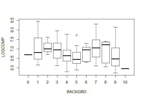
Professional background (BACKGRD) of the CEO contains eleven categories, such as marketing, finance, accounting, insurance and so on. We use this factor to explain logarithmic compensation (LOGCOMP).
IV.1. The number and mean effects of BACKGRD on LOGCOMP are described in the table below. A boxplot is given in Figure 1. Describe what we learn from the table and boxplot about the effect of BACKGRD on LOGCOMP.
> cbind(summarize(LOGCOMP,BACKGRD,length),
+      round(summarize(LOGCOMP,BACKGRD,mean,na.rm=TRUE),digits=3))
   BACKGRD LOGCOMP BACKGRD LOGCOMP
       0       1       0   6.690
       1      17       1   7.064
       2       3       2   7.103
       3      13       3   6.916
       4      13       4   6.679
       5      12       5   6.553
       6       7       6   6.764
       7      12       7   7.067
       8       6       8   6.914
       9      14       9   6.621
      10       1      10   5.956
> boxplot(LOGCOMP~EDUCATN,ylab="LOGCOMP",xlab="EDUCATN")
Solution
IV.2. Consider a regression model using only the factor, BACKGRD; the fitted output is below.
- a. Provide an expression for the regression function for this model, defining each term.
- b. Provide an expression for the fitted regression function, using the fitted output. Further, give the fitted value for an observation with BACKGRD = 0 and with BACKGRD = 1, both in logarithmic units as well as dollars.
- c. Is BACKGRD a statistically significant determinant of LOGCOMP? State your null and alternative hypotheses, decision-making criterion, and your decision-making rules. (Hint: Use the R2 statistic to compute an F-statistic.)
> summary(lm(LOGCOMP ~ factor(BACKGRD)))

Call:
lm(formula = LOGCOMP ~ factor(BACKGRD))

Coefficients:
                  Estimate Std. Error t value Pr(>|t|)
(Intercept)        6.68960    0.60605  11.038   <2e-16 ***
factor(BACKGRD)1   0.37441    0.62362   0.600    0.550
factor(BACKGRD)2   0.41388    0.69980   0.591    0.556
factor(BACKGRD)3   0.22644    0.62892   0.360    0.720
factor(BACKGRD)4  -0.01012    0.62892  -0.016    0.987
factor(BACKGRD)5  -0.13649    0.63079  -0.216    0.829
factor(BACKGRD)6   0.07449    0.64789   0.115    0.909
factor(BACKGRD)7   0.37771    0.63079   0.599    0.551
factor(BACKGRD)8   0.22431    0.65461   0.343    0.733
factor(BACKGRD)9  -0.06845    0.62732  -0.109    0.913
factor(BACKGRD)10 -0.73376    0.85708  -0.856    0.394
---
Signif. codes:  0 ‘***’ 0.001 ‘**’ 0.01 ‘*’ 0.05 ‘.’ 0.1 ‘ ’ 1

Residual standard error: 0.606 on 88 degrees of freedom
Multiple R-squared: 0.1248,     Adjusted R-squared: 0.0253
Part V. Variable Selection.
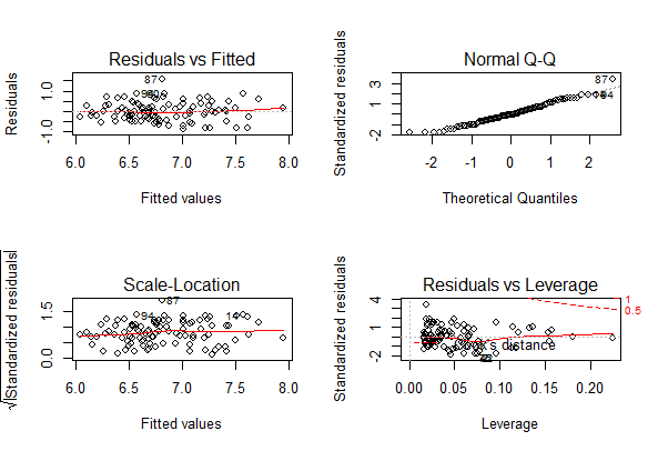
V.1 We run a regression model using LOGCOMP as the outcome of interest and four explanatory variables, LOGSALES, GRAD, PERCENT5, and EXPER. In Figure 2 is a set of four diagnostic plots of this model.
- a. In the upper left-hand panel is a plot of residuals versus fitted values. What type of model misspecification does this type of plot help detect?
- b. Does the plot of residuals versus fitted values in Figure 2 reveal a serious model misspecification?
- c. In the upper right-hand panel is a normal qq-plot. Describe this plot and say what type of model misspecification it helps to detect.
- d. Does the normal qq-plot in Figure 2 reveal a serious model misspecification?
- e. In the lower right-hand panel is a plot of standardized residuals versus leverages. Describe this plot and say what type of model misspecification it helps to detect.
- f. Observation 87 appears in Figure 2. Is it a high leverage point? Describe the average leverage for this data set and give a rule of thumb cut-off for a point to be a high leverage point.
- g. Observation 87 appears in Figure 2. Is it an outlier? Give a rule of thumb cut-off for a point to be an outlier.
Solution
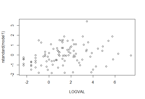
V.2 We run a regression model using LOGCOMP as the outcome of interest and four explanatory variables, LOGSALES, GRAD, PERCENT5, and EXPER. In Figure 3 is a plot of LOGVAL versus the residuals from this model. The correlation between these two variables is 0.292.
- a. What do we hope to learn from a plot of a potential explanatory variable versus residuals from a model fit?
- b. What new model does the information in Figure 3 suggest that we specify?
Solution
Part VI. Some Algebra Problems.
VI.1 Regression through the origin. Consider the model (y_i=beta_1 z_i^2 + varepsilon_i), a quadratic model passing through the origin.
- a. Determine the least squares estimate of (beta_1).
- b. Using the following set of n=5 observations, given a numerical result for the least squares estimate of (beta_1) determined in part (a).
begin{equation*}
begin{array}{l|rrrrr}
hline
i & 1 & 2 & 3 & 4 & 5 \
z_i & -2 & -1 & 0 & 1 & 2 \
y_i & 4 & 0 & 0 & 1 & 4 \ hline
end{array}
end{equation*}
Solution
VI.2 You are doing regression with one explanatory variable and so consider the basic linear regression model (y_i = beta_0 + beta_1 x_i + varepsilon_i).
- a. Show that the ith leverage can be simplified to
begin{equation*}
h_{ii} = frac{1}{n} + frac{(x_i - overline{x})^2}{(n-1) s_x^2}.
end{equation*} - b. Show that (overline{h}= 2 / n).
- c. Suppose that (h_{ii} = 6/n) . How many standard deviations is (x_i) away (either above or below) from the mean?