An investor’s decision to purchase a stock is generally made with a number of criteria in mind. First, investors usually look for a high expected return. A second criterion is the riskiness of a stock which can be measured through the variability of the returns. Third, many investors are concerned with the length of time that they are committing their capital with the purchase of a security. Many income stocks, such as utilities, regularly return portions of capital investments in the form of dividends. Other stocks, particularly growth stocks, return nothing until the sale of the security. Thus, the average length of investment in a security is another criterion. Fourth, investors are concerned with the ability to sell the stock at any time convenient to the investor. We refer to this fourth criterion as the liquidity of the stock. The more liquid is the stock, the easier it is to sell. To measure the liquidity, in this study we use the number of shares traded on an exchange over a specified period of time (called the VOLUME). We are interested in studying the relationship between the volume and other financial characteristics of a stock.
We begin this study with 126 companies whose options were traded on December 3, 1984. The stock data were obtained from Francis Emory Fitch, Inc. for the period from December 3, 1984 to February 28, 1985. For the trading activity variables, we examine
- the three months total trading volume (VOLUME, in millions of shares),
- the three months total number of transactions (NTRAN), and
- the average time between transactions (AVGT, measured in minutes).
For the firm size variables, we use the
- opening stock price on January 2, 1985 (PRICE),
- the number of outstanding shares on December 31, 1984 (SHARE, in millions of shares), and
- the market equity value (VALUE, in billions of dollars) obtained by taking the product of PRICE and SHARE.
Finally, for the financial leverage, we examine the debt-to-equity ratio (DEB_EQ) obtained from the Compustat Industrial Tape and the Moody’s manual. The data in SHARE are obtained from the Center for Research in Security Prices (CRSP) monthly tape.
After examining some preliminary summary statistics of the data, three companies were deleted because they either had an unusually large volume or high price. They are Teledyne and Capital Cities Communication, whose prices were more than four times the average price of the remaining companies, and American Telephone and Telegraph, whose total volume was more than seven times than the average total volume of the remaining companies. Based on additional investigation, the details of which are not presented here, these companies were deleted because they seemed to represent special circumstances that we would not wish to model. Table 5.2 summarizes the descriptive statistics based on the remaining n=123 companies. For example, from Table 5.2 we see that the average time between transactions is about five minutes and this time ranges from a minimum of less than a minute to a maximum of about 20 minutes.
begin{matrix}begin{array}{c}
text{Table 5.2 Summary Statistics of the Stock Liquidity Variables}
end{array}\small
begin{array}{lrrrrr} hline & & & text{Standard} & & \ & text{Mean} & text{Median} & text{deviation} & text{Minimum} & text{Maximum} \ hline text{VOLUME} & 13.423 & 11.556 & 10.632 & 0.658 & 64.572 \ text{AVGT} & 5.441 & 4.284 & 3.853 & 0.590 & 20.772 \ text{NTRAN} & 6436 & 5071 & 5310 & 999 & 36420 \ PRICE & 38.80 & 34.37 & 21.37 & 9.12 & 122.37 \ text{SHARE} & 94.7 & 53.8 & 115.1 & 6.7 & 783.1 \ text{VALUE} & 4.116 & 2.065 & 8.157 & 0.115 & 75.437 \ text{DEB_EQ} & 2.697 & 1.105 & 6.509 & 0.185 & 53.628 \ hline end{array}\scriptsize
begin{array}{c}
Source: text{Francis Emory Fitch, Inc., Standard & Poor’s Compustat,}\ text{ and University of Chicago’s Center for Research on Security Prices.}
end{array}
end{matrix}
R Code for Table 5.2
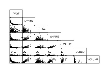
Table 5.3 reports the correlation coefficients and Figure 5.2 provides the corresponding scatterplot matrix. If you have a background in finance, you will find it interesting to note that the financial leverage, measured by DEB_EQ, does not seem to be related to the other variables. From the scatterplot and correlation matrix, we see a strong relationship between VOLUME and the size of the firm as measured by SHARE and VALUE. Further, the three trading activity variables, VOLUME, AVGT and NTRAN, are all highly related to one another.
begin{matrix}
begin{array}{c}
text{Table 5.3 Correlation Matrix of the Stock Liquidity}
end{array}\small
begin{array}{lrrrrrrr} hline & text{AVGT} & text{NTRAN} & text{PRICE} & text{SHARE} & text{VALUE} & text{DEB_EQ} \ hline text{NTRAN} & -0.668 & & & & & \ text{PRICE} & -0.128 & 0.190 & & & & \ text{SHARE} & -0.429 & 0.817 & 0.177 & & & \ text{VALUE} & -0.318 & 0.760 & 0.457 & 0.829 & & \ text{DEB_EQ} & 0.094 & -0.092 & -0.038 & -0.077 & -0.077 & \ text{VOLUME} & -0.674 & 0.913 & 0.168 & 0.773 & 0.702 & -0.052 \ hline end{array} end{matrix}
R Code for Table 5.3
Figure 5.2 shows that the variable AVGT is inversely related to VOLUME and NTRAN is inversely related to AVGT. In fact, it turned out the correlation between the average time between transactions and the reciprocal of the number of transactions was (99.98%)! This is not so surprising when one thinks about how AVGT might be calculated. For example, on the New York Stock Exchange, the market is open from 10:00 A.M. to 4:00 P.M. For each stock on a particular day, the average time between transactions times the number of transactions is nearly equal to 360 minutes (= 6 hours). Thus, except for rounding errors because transactions are only recorded to the nearest minute, there is a perfect linear relationship between AVGT and the reciprocal of NTRAN.
R Code for Figure 5.2
To begin to understand the liquidity measure VOLUME, we first fit a regression model using NTRAN as an explanatory variable. The fitted regression model is:
begin{matrix} begin{array}{lccl} text{VOLUME} & = & 1.65 & +0.00183 text{NTRAN} \ text{std errors} & & (0.0018) & (0.000074) \ end{array} end{matrix}
R Code for Regression
with (R^2=83.4%) and (s=4.35). Note that the t-ratio for the slope associated with NTRAN is (t(b_1)=b_1/se(b_1)) = 0.00183/0.000074 = 24.7, indicating strong statistical significance. Residuals were computed using this estimated model. To see if the residuals are related to the other explanatory variables, below is a table of correlations.
begin{matrix}begin{array}{c}
text{Table 5.4 First Table of Correlations}
end{array}\small
begin{array}{cccccc} hline & text{AVGT} & text{PRICE} & text{SHARE} & text{VALUE} & text{DEB_EQ} \ text{RESID} & -0.155 & -0.017 & 0.055 & 0.007 & 0.078 \ hline end{array} \scriptsize
begin{array}{c}
Note:text{ The residuals were created from a regression of VOLUME on NTRAN.}
end{array} end{matrix}
R Code for Table 5.4
The correlation between the residual and AVGT and the scatter plot (not given here) indicates that there may be some information in the variable AVGT in the residual. Thus, it seems sensible to use AVGT directly in the regression model. Remember that we are interpreting the residual as the value of VOLUME having controlled for the effect of NTRAN.
We next fit a regression model using NTRAN and AVGT as an explanatory variables. The fitted regression model is:
begin{matrix} begin{array}{lccll} text{VOLUME} & = & 4.41 & -0.322 text{AVGT} & +0.00167 text{NTRAN} \ text{std errors} & & (1.30) & (0.135) & (0.000098) \ end{array} end{matrix}
R Code for Regression
with (R^2=84.2%) and s=4.26. Based on the t-ratio for AVGT, (t(b_{AVGT})=) (-0.322)/0.135 =-2.39, it seems as if AVGT is a useful explanatory variable in the model. Note also that s has decreased, indicating that (R_a^2) has increased.
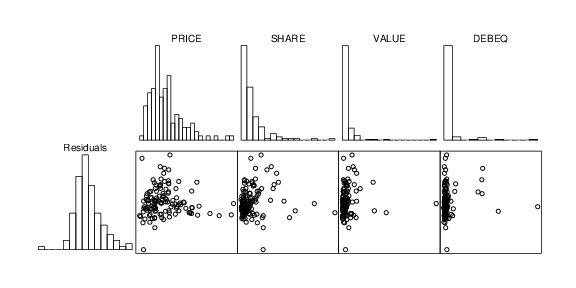
Table 5.5 provides correlations between the model residuals and other potential explanatory variables and indicates that there does not seem to be much additional information in the explanatory variables. This is reaffirmed by the corresponding table of scatter plots in Figure 5.3. The histograms in Figure 5.3 suggest that although the distribution of the residuals is fairly symmetric, the distribution of each explanatory variable is skewed. Because of this, transformations of the explanatory variables were explored. This line of thought provided no real improvements and thus the details are not provided here.
R Code for Figure 5.3
begin{matrix}begin{array}{c}
text{Table 5.5 Second Table of Correlations}
end{array}\scriptsize
begin{array}{ccccc} hline & text{PRICE} & text{SHARE} & text{VALUE} & text{DEB_EQ} \ text{RESID} & -0.015 & 0.096 & 0.071 & 0.089 \ hline end{array} \scriptsize
begin{array}{c}
Note:text{ The residuals were created from a regression of VOLUME on NTRAN and AVGT.}
end{array}end{matrix}