We now study the impact of various predictors on hospital charges in the state of Wisconsin. Identifying predictors of hospital charges can provide direction for hospitals, government, insurers and consumers in controlling these variables that in turn leads to better control of hospital costs. The data for the year 1989 were obtained from the Office of Health Care Information, Wisconsin’s Department of Health and Human Services. Cross sectional data are used, which details the 20 diagnosis related group (DRG) discharge costs for hospitals in the state of Wisconsin, broken down into nine major health service areas and three types of providers (Fee for service, HMO, and other). Even though there are 540 potential DRG, area and payer combinations ((20times 9times 3=540)), only 526 combinations were actually realized in the 1989 data set. Other predictor variables included the logarithm of the total number of discharges (NO DSCHG) and total number of hospital beds (NUM BEDS) for each combination. The response variable is the logarithm of total hospital charges per number of discharges (CHGNUM). To streamline the presentation, we now consider only costs associated with three diagnostic related groups (DRGs), DRG #209, DRG #391 and DRG #430.
The covariate, x, is the natural logarithm of the number of discharges. In ideal settings, hospitals with more patients enjoy lower costs due to economies of scale. In non-ideal settings, hospitals may not have excess capacity and thus, hospitals with more patients have higher costs. One purpose of this analysis is to investigate the relationship between hospital costs and hospital utilization.
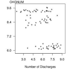
Recall that our measure of hospital charges is the logarithm of costs per discharge y. The scatter plot in Figure 4.6 gives a preliminary idea of the relationship between y and x. We note that there appears to be a negative relationship between y and x.
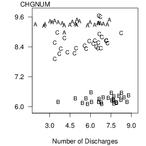
The negative relationship between y and x suggested by Figure 4.6 is misleading and is induced by an omitted variable, the category of the cost (DRG). To see the joint effect of the categorical variable DRG and the continuous variable x, in Figure 4.7 is a plot of y versus x where the plotting symbols are codes for the level of the categorical variable. From this plot, we see that the level of cost varies by level of the factor DRG. Moreover, for each level of DRG, the slope between y and x is either zero or positive. The slopes are not negative, as suggested by Figure 4.6.
R Code for Figure 4.6
begin{matrix}begin{array}{c}
text{Table 4.8 Wisconsin Hospital Cost Models Goodness of Fit.}
end{array}\scriptsize
begin{array}{lccrcc} hline & text{Model} & text{Error} & text{Error} & & text{Error} \ & text{degrees} & text{degrees} & text{Sum} & R^2 & text{Mean} \ text{Model Description} & text{of freedom} & text{of freedom} & text{of Squares} & (%) & text{Square} \ hline text{One factor ANOVA} & 2 & 76 & {9.396} & { 93.3} & {0.124} \ text{Regression with constant intercept} & 1 & 77 & {115.059} & {18.2} & {1.222} \ ~~~text{and slope} & & & & & \ text{Regression with variable intercept} &3 & 75 & {7.482} & 94.7 & {0.100} \ ~~~text{and constant slope} & & & & & \ text{Regression with constant intercept} & 3 & 75 & {14.048} & {90.0} & {0.187} \ ~~~text{and variable slope} & & & & & \ text{Regression with variable intercept} & 5 & 73 & {5.458} & {96.1} & {0.075} \ ~~~text{and slope} & & & & & \ hline end{array}\scriptsize
begin{array}{l}Note: text{These models represent combinations of one factor and one covariate.} \ end{array}
end{matrix}
Each of the five models defined in Table 4.7 was fit to this subset of the Hospital case study. The summary statistics are in Table 4.8. For this data set, there are (n=79) observations and c=3 levels of the DRG factor. For each model, the model degrees of freedom is the number of model parameters minus one. The error degrees of freedom is the number of observations minus the number of model parameters.
Using binary variables, each of the models in Table 4.7 can be written in a regression format. As we have seen in Section 4.2, when a model can be written as a subset of another, larger model, we have formal testing procedures available to decide which model is more appropriate. To illustrate this testing procedure with our DRG example, from Table 4.8 and the associated plots, it seems clear that the DRG factor is important. Further, a t-test, not presented here, shows that the covariate x is important. Thus, let’s compare the full model E (y_{ij} = beta_{0,j} + beta_{1,j}x) to the reduced model E (y_{ij}=beta_{0,j}+beta_1x). In other words, is there a different slope for each DRG?
Using the notation from Section 4.2, we call the variable intercept and slope the full model. Under the null hypothesis, (H_0: beta_{1,1}=beta_{1,2}=beta_{1,3}), we get the variable intercept, constant slope model. Thus, using the (F)-ratio in equation (4.2), we have begin{equation*} Ftext{-ratio}=frac{(Error~SS)_{reduced}-(Error~SS)_{full}}{ps_{full}^2}=frac{{7.482-5.458}}{2(0.075)}=13.535. end{equation*} The 95(th) percentile from the F-distribution with (df_1=p=2) and (df_2=(df)_{full})=73 is approximately 3.13. Thus, this test leads us to reject the null hypothesis and declare the alternative, the regression model with variable intercept and variable slope, to be valid.