We now return to the marital status of respondents from the Survey of Consumer Finances (SCF). Recall that marital status is not measured continuously but rather takes on values that falls into distinct groups that we treat as unordered. In Chapter 3, we grouped survey respondents according to whether or not they are “single,” where being single includes never married, separated, divorced, widowed, and are not married and living with a partner. We now supplement this by considering the categorical variable, MARSTAT, that represents the marital status of the survey respondent. This may be:
- 1, for married
- 2, for living with partner
- 0, for other (SCF further breaks down this category into separated, divorced, widowed, never married and inapplicable, persons age 17 or less, no further persons).
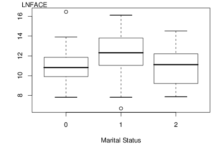
As before, the dependent variable is y = LNFACE, the amount that the company will pay in the event of the death of the named insured (in logarithmic dollars). Table 4.1 summarizes the dependent variable by level of the categorial variable. This table shows that the marital status “married” is the most prevalent in the sample and that those married choose to have the most life insurance coverage. Figure 4.1 gives a more complete picture of the distribution of LNFACE for each of the three types of marital status. The table and figure also suggests that those living together have less life insurance coverage than the other two categories.
begin{matrix}begin{array}{c}
text{Table 4.1 Summary Statistics of Logarithmic Face By Marital Status}
end{array}\small
begin{array}{lcccc} hline & & & & text{Standard} \ & text{MARSTAT} & text{Number} & text{Mean} & text{deviation}\hline text{Other} & 0 & 57 & 10.958 & 1.566 \ text{Married} & 1 & 208 & 12.329 & 1.822 \ text{Living together} & 2 & 10 & 10.825 & 2.001 \ hline text{Total} & & 275 & 11.990 & 1.871 \ hline end{array} end{matrix}
R Code for Table 4.1
R Code for Figure 4.1
Are the continuous and categorical variables jointly important determinants of response? To answer this, a regression was run using LNFACE as the response and five explanatory variables, three continuous and two binary (for marital status). Recall that our three continuous explanatory variables are: LNINCOME (logarithmic annual income), the number of years of EDUCATION of the survey respondent and the number of household members, NUMHH.
For the binary variables, first define MAR0 to be the binary variable that is one if MARSTAT=0 and zero otherwise. Similarly, define MAR1 and MAR2 to be binary variables that indicate MARSTAT=1 and MARSTAT=2, respectively. There is a perfect linear dependency among these three binary variables in that MAR0 + MAR1 + MAR2 = 1 for any survey respondent. Thus, we need only two of the three. However, there is not a perfect dependency among any two of the three. It turns out that Corr(MAR0,MAR1) = -0.90, Corr(MAR0,MAR2) =-0.10 and Corr(MAR1,MAR2) = -0.34.
R Code to Compute Correlation
A regression model was run using LNINCOME, EDUCATION, NUMHH, MAR0 and MAR2 as explanatory variables. The fitted regression equation turns out to be begin{eqnarray*} widehat{y} &=& 2.605 + 0.452 textrm{LNINCOME} +0.205 textrm{EDUCATION} + 0.248 textrm{NUMHH} \ & & ~~ -0.557 textrm{MAR0} -0.789 textrm{MAR2}. end{eqnarray*}
R Code for Regression
To interpret the regression coefficients associated with marital status, consider a respondent who is married. In this case, then MAR0=0, MAR1=1 and MAR2=0, so that begin{eqnarray*} widehat{y}_m &=& 2.605 + 0.452 textrm{LNINCOME} +0.205 textrm{EDUCATION} + 0.248 textrm{NUMHH} . end{eqnarray*} Similarly, if the respondent is coded as living together, then MAR0=0, MAR1=0 and MAR2=1, and
begin{align} widehat{y}_{lt} &= 2.605 + 0.452 textrm{LNINCOME} +0.205 textrm{EDUCATION} + 0.248 textrm{NUMHH}\ &-0.789. end{align} The difference between (widehat{y}_m) and (widehat{y}_{lt}) is (0.789.) Thus, we may interpret the regression coefficient associated with MAR2, -0.789, to be the difference in fitted values for someone living together compared to a similar person who is married (the omitted category).
Similarly, we can interpret -0.557 to be the difference between the ``other'' category and the married category, holding other explanatory variables fixed. For the difference in fitted values between the ``other'' and the ``living together'' categories, we may use (-0.557 - (-0.789) = 0.232.)
Although the regression was run using MAR0 and MAR2, any two out of the three would produce the same ANOVA Table 4.2. However, the choice of binary variables does impact the regression coefficients. Table 4.3 shows three models, omitting MAR1, MAR2 and MAR0, respectively. For each fit, the coefficients associated with the continuous variables remain the same. As we have seen, the binary variable interpretations are with respect to the omitted category, known as the reference level. Although they change from model to model, they overall interpretation remains the same. That is, if we would like to estimate the difference in coverage between the ``other'' and the ``living together'' category, the estimate would be 0.232, regardless of the model.
begin{matrix}begin{array}{c}
text{Table 4.2 Term Life with Marital Status ANOVA Table}
end{array}\small
begin{array}{lrrr} hline text{Source} & text{Sum of Squares} & df & text{Mean Square} \ hline
text{Regression} & 343.28 & 5 & 68.66 \ text{Error} & 615.62 & 269 & 2.29 \ text{Total} & 948.90& 274 & \ hline
end{array}\scriptsize
begin{array}{l}
text{Residual Standard Error} s= 1.513, R^2 = 35.8%, R_a^2 = 34.6%end{array} end{matrix}
R Code for Table 4.2
Although the three models in Table 4.3 are the same except for different choices of parameters, they do appear different. In particular, the (t)-ratios differ and give different appearances of statistical significance. For example, both of the (t)-ratios associated with marital status in Model 2 are less than 2 in absolute value, suggesting that marital status is unimportant. In contrast, both Models 1 and 3 have at least one marital status binary that exceeds 2 in absolute value, suggesting statistical significance. Thus, you can influence the appearance of statistical significance by altering the choice of the reference level. To assess the overall importance of marital status (not just each binary variable),
Section 4.2 will introduce tests of sets of regression coefficients.
begin{matrix}begin{array}{c}
text{Table 4.3 Term Life Regression Coefficients with Marital Status}
end{array}\scriptsize
begin{array}{llll}
hline phantom{XXXXXXXXXXX} & text{Model 1}phantom{XXXXX}& phantom{XX}text{Model 2}phantom{XXXXX}& phantom{XX}text{Model 3}phantom{XXXXX}\
end{array}\scriptsize
begin{array}{l|rr|rr|rr} hline text{Explanatory} \ text{Variable} & text{Coefficient} & t-text{ratio} & text{Coefficient} & t-text{ratio}& text{Coefficient} & t-text{ratio}\hline text{LNINCOME} & 0.452 & 5.74 & 0.452 & 5.74 & 0.452 & 5.74 \ text{EDUCATION} &0.205 & 5.30 &0.205 & 5.30&0.205 & 5.30 \ text{NUMHH} & 0.248 & 3.57 & 0.248 & 3.57 & 0.248 & 3.57 \hline text{Intercept} & 3.395 & 3.77 & 2.605& 2.74 & 2.838 & 3.34\ text{MAR0} & -0.557 & -2.15& 0.232 & 0.44\ text{MAR1} & & & 0.789 & 1.59 & 0.557 & 2.15\ text{MAR2} & -0.789 & -1.59 & & & -0.232 & -0.44\ hline end{array}
end{matrix}
R Code for Table 4.3