In some applications, we expect the response to have some abrupt changes in behavior at certain values of an explanatory variable, even if the variable is continuous. For example, suppose that we are trying to model an individual’s charitable contributions (y) in terms of their wages (x). For 2007 data, a simple model we might entertain is given in Figure 3.9.
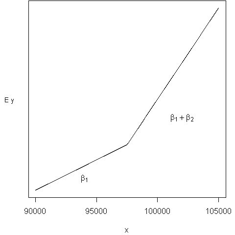
Figure 3.9. The marginal change in E y is lower below $97,500. The parameter (beta_2) represents the difference in the slopes.
A rational for this model is that, in 2007 individuals paid 7.65% of their income for Social Security taxes up to $97,500. No social security taxes are excised on wages in excess of $97,500. Thus, one theory is that, for wages in excess of $97,500, individuals have more disposal income per dollar and thus should be more willing to make charitable contributions.
To model this relationship, define the binary variable x to be zero if x < 97,500 and to be one if x (geq) 97,500. Define the regression function to be E (y = beta_0 + beta_1 x + beta_2 z (x – 97,500).) This can be written as:
begin{equation*} text{E }y = left{ begin{array}{ll} beta_0 + beta_1 x & x < 97,500 \ beta_0 - beta_2(97,500) + (beta_1+beta_2) x & x geq 97,500 end{array} . right. end{equation*} To estimate this model, we would run a regression of y on two explanatory variables, (x_1 = x) and (x_2 = z times (x – 97,500)). If (beta_2 > 0,) then the marginal rate of charitable contributions is higher for incomes exceeding $97,500.
Figure 3.9 illustrates this relationship, known as piecewise linear regression or sometimes a “broken stick” model. The sharp break in Figure 3.9 at (x = 97,500) is called a “kink.” We have linear relationships above and below the kinks and have used a binary variable to put the two pieces together. We are not restricted to one kink. For example, suppose that we wish to do a historical study of Federal taxable income for 1992 single filers. Then, there were three tax brackets: the marginal tax rate below $21,450 was 15%, above $51,900 was 31%, and in between was 28 percent. For this example, we would use two kinks, at 21,450 and 51,900.
Further, piecewise linear regression is not restricted to continuous response functions. For example, suppose that we are studying the commissions paid to stockbrokers (y) in terms of the number of shares purchased by a client (x). We might expect to see the relationship illustrated in Figure 3.10. Here, the discontinuity at x = 100 reflects the administrative expenses of trading in odd lots, as trades of less than 100 shares are called. The lower marginal cost for trades in excess of 100 shares simply reflects the economies of scale for doing business in larger volumes. A regression model of this is E (y = beta_0 + beta_1 x + beta_2 z + beta_3 z x) where z = 0 if x ( < ) 100 and z = 1 if x (geq) 100. The regression function depicted in Figure 3.10 is
begin{equation*} text{E }y = left{ begin{array}{ll} beta_0 + beta_1 x_1 & x<100 \ beta_0 + beta_2 + (beta_1+beta_3) x_1 & x geq 100 end{array} . right. end{equation*}
[caption id="attachment_269" align="aligncenter" width="300"]
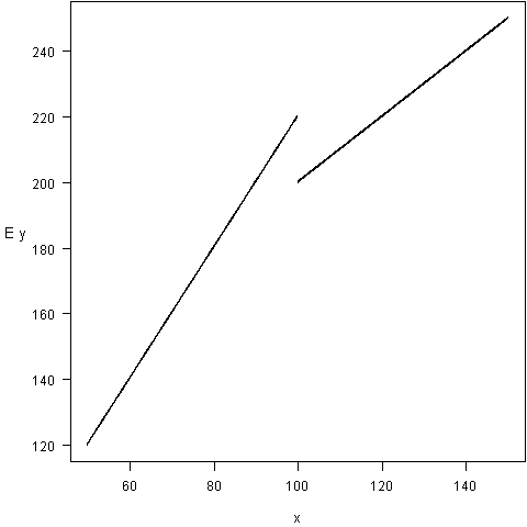
Figure 3.10. Plot of expected commissions (E y) versus number of shares traded (x). The break at (x=100) reflects savings in administrative expenses. The lower slope for (x geq 100) reflects economies of scales in expenses. [/caption]