For completeness, here are a few definitions. The sample is the set of data available for analysis, denoted by $(y_1,\ldots,y_n$). Here, ($n$) is the number of observations, ($y_1$) represents the first observation, $(y_2$) the second, and so on up to ($y_n$) for the ($n$th) observation. Here are a few important summary statistics.
- The mean is the average of observations, that is, the sum of the observations divided by the number of units. Using algebraic notation, the mean is $\overline{y}=\frac{1}{n}\left( y_1 + \cdots + y_n \right) = \frac{1}{n} \sum_{i=1}^{n} y_i.$
- The median is the middle observation when the observations are ordered by size. That is, it is the observation at which 50% are below it (and 50% are above it).
- The standard deviation is a measure of the spread, or scale, of the distribution. It is computed as $s_y = \sqrt{\frac{1}{n-1}\sum_{i=1}^{n}\left( y_i-\overline{y}\right)^{2}} .$
- A percentile is a number at which a specified fraction of the observations is below it, when the observations are ordered by size. For example, the 25th percentile is that number so that 25% of observations are below it.
To help visualize the distribution, Figure 1.2 displays a histogram of the data. Here, the height of the each rectangle shows the relative frequency of observations that fall within the range given by its base. The histogram provides a quick visual impression of the distribution; it shows that the range of the data is approximately (-4,4), the central tendency is slightly greater than zero and that the distribution is roughly symmetric.
Normal Curve Approximation. Figure 1.2 also shows a normal curve superimposed, using ($\overline{y}$) for ($\mu$ ) and ($s_y^{2}$) for ($\sigma ^{2}$). With the normal curve, only two quantities (($\mu$ ) and ($\sigma ^{2}$)) are required to summarize the entire distribution. For example, Table 1.2 shows that 1.168 is the 75th percentile, which is approximately the 204th (= .75 (times) 272) largest observation from the entire sample. From the normal distribution, we have that ($z=(y-\mu )/\sigma$ ) is a standard normal, of which 0.675 is the 75th percentile. Thus, ($\overline{ y}+0.675s_y)=0.481+0.675(\times) 1.101=1.224$ is the 75th percentile using the normal curve approximation.
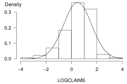
Figure 1.2. Bodily Injury Relative Frequency with Normal Curve Superimposed.