- Calculate probabilities under a standard normal curve
- Calculate and interpret five basic summary statistics
- Fit a data set to a normal curve
- Calculate and interpret Box and qq– Plots
Video Overview of the Section (Alternative .mp4 Version – 11:49 min)
Historically, the normal distribution had a pivotal role in the development of regression analysis. It continues to play an important role, although we will be interested in extending regression ideas to highly “non-normal” data.
Formally, the normal curve is defined by the function \begin{equation} \mathrm{f}(y)=\frac{1}{\sigma \sqrt{2\pi }}\exp \left( -\frac{1}{2\sigma^{2} }\left( y-\mu \right)^{2}\right) . \end{equation}
This curve is a probability density function with the whole real line as its domain. From equation (1.1), we see that the curve is symmetric about ($\mu$) (the mean and median). The degree of peakedness is controlled by the parameter ($\sigma ^{2}$). These two parameters, ($\mu$ ) and ($\sigma^{2}$), are known as the location and scale parameters, respectively. Appendix A3.1 provides additional details about this curve, including a graph and tables of its cumulative distribution that we will use throughout the text.
The normal curve is also depicted in Figure 1.1, a display of a now out-of-date German currency note, the ten Deutsche Mark. This note contains the image of German Carl Gauss, an eminent mathematician whose name is often linked with the normal curve (it is sometimes referred to as the Gaussian curve). Gauss developed the normal curve in connection with the theory of least squares for fitting curves to data in 1809, about the same time as related work by the French scientist Pierre LaPlace. According to Stigler (1986), there was quite a bit of acrimony between these two scientists about the priority of discovery! The normal curve was first used as an approximation to histograms of data around 1835 by Adolph Quetelet, a Belgian mathematician and social scientist. Like many good things, the normal curve had been around for some time, since about 1720 when Abraham de Moivre derived it for his work on modeling games of chance. The normal curve is popular because it is easy to use and has proved to be successful in many applications.
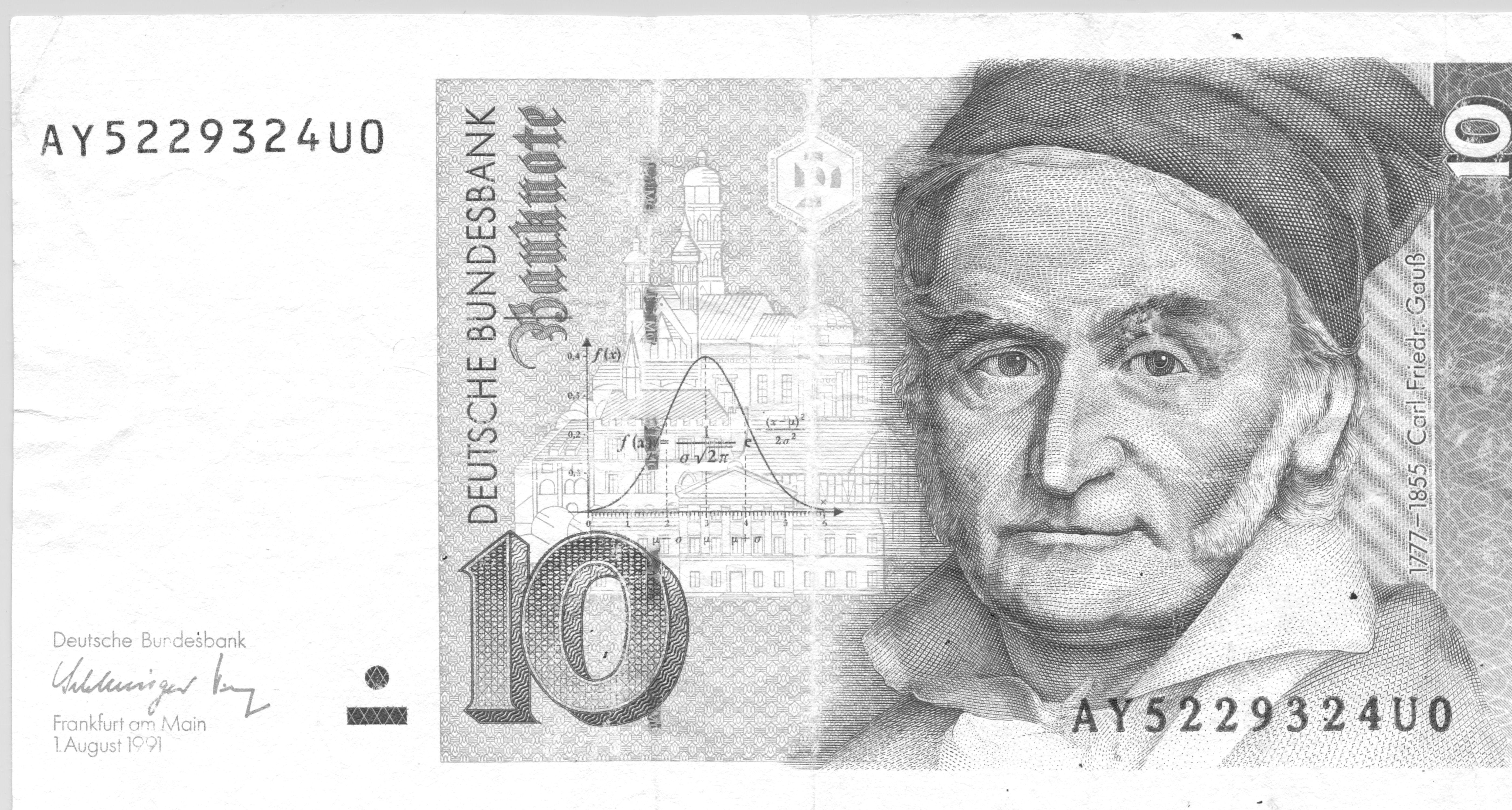
Figure 1.1. Ten Deutsche Mark – German currency featuring scientist Gauss and the normal curve .