- Explain the logic behind why regression coefficients are weighted sums and how this helps us understand their sampling distributions
- Interpret the coefficients as unbiased
- Explain the variance of the sampling distribution of regression coefficients
- Define the standard error of a regression coefficient
- Interpret the behavior of a regression coefficient’s standard error
Video Overview of the Section (Alternative .mp4 Version – 7:37 min)
The exercises ask the reader to verify that (b_0) can also be expressed as a weighted sum of responses, so our discussion pertains to both regression coefficients. Because regression coefficients are weighted sums of responses, they can be affected dramatically by unusual observations (see Section 2.6).
Because (b_1) is a weighted sum, it is straightforward to derive the expectation and variance of this statistic. By the linearity of expectations and Assumption F1, we have begin{equation*} mathrm{E}~b_1=sum_{i=1}^{n}w_i~mathrm{E}~y_i=beta_0sum_{i=1}^{n}w_i+beta_1sum_{i=1}^{n}w_ix_i=beta_1. end{equation*} That is, (b_1) is an unbiased estimator of (beta_1). Here, the sum ( sum_{i=1}^{n}w_ix_i) (=) (left[ s_x^2(n-1)right] ^{-1}sum_{i=1}^{n}left( x_i-overline{x}right) x_i) (=left[ s_x^2(n-1)right] ^{-1}sum_{i=1}^{n}left( x_i-overline{x}right) ^2=1.) From the definition of the weights, some easy algebra also shows that (sum_{i=1}^{n}w_i^2=1/left( s_x^2(n-1)right) ). Further, the independence of the responses implies that the variance of the sum is the sum of the variances, and thus we have begin{equation*} mathrm{Var}~b_1=sum_{i=1}^{n}w_i^2mathrm{Var}~y_i=frac{sigma ^2}{s_x^2(n-1)}. end{equation*} Replacing (sigma ^2) by its estimator (s^2) and taking square roots leads to the following.
Definition. The standard error of (b_1), the estimated standard deviation of (b_1), is defined as begin{equation} se(b_1)=frac{s}{s_xsqrt{n-1}}. label{seb1a} end{equation}
This is our measure of the reliability, or precision, of the slope estimator. Using equation (2.5), we see that (se(b_1)) is determined by three quantities, (n), (s) and (s_x), as follows:
- If we have more observations so that (n) becomes larger, then ( se(b_1)) becomes smaller, other things equal.
- If the observations have a greater tendency to lie closer to the line so that (s) becomes smaller, then (se(b_1)) becomes smaller, other things equal.
- If values of the explanatory variable become more spread out so that ( s_x) increases, then (se(b_1)) becomes smaller, other things equal.
Smaller values of (se(b_1)) offer a better opportunity to detect relations between (y) and (x). Figure 2.5 illustrates these relationships. Here, the scatter plot in the middle has the smallest value of (se(b_1)). Compared with the middle plot, the left-hand plot has a larger value of (s) and thus (se(b_1)). Compared with the right-hand plot, the middle plot has a larger (s_x), and thus smaller value of (se(b_1)).
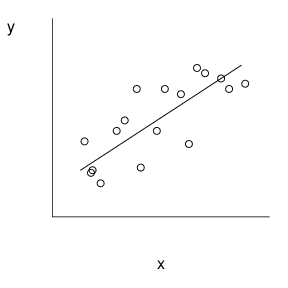
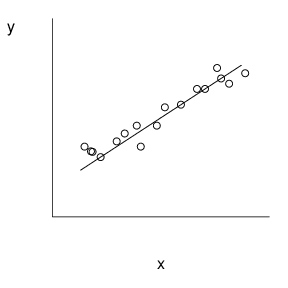
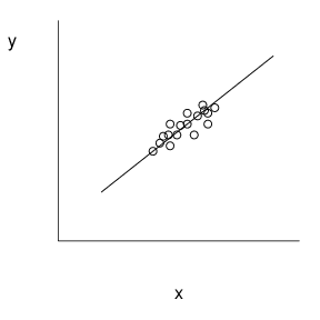
Figure 2.5 These three scatter plots exhibit the same linear relationship between (y) and (x). The plot on the top exhibits greater variability about the line than the plot in the middle. The plot on the bottom exhibits a smaller standard deviation in (x) than the plot in the middle.
R Code for Figure 2.5
Equation (2.4) also implies that the regression coefficient (b_1 ) is normally distributed. That is, recall from mathematical statistics that linear combinations of normal random variables are also normal. Thus, if Assumption F5 holds, then (b_1) is normally distributed. Moreover, several versions of central limit theorems exists for weighted sums (see, for example, Serfling, 1980). Thus, as discussed in Section 1.4, if the responses (y_i) are even approximately normally distributed, then it will be reasonable to use a normal approximation for the sampling distribution of (b_1). Using (se(b_1)) as the estimated standard deviation of (b_1), for large values of (n) we have that (left( b_1-beta_1right) /se(b_1)) has an approximate standard normal distribution. Although we will not prove it here, under Assumption F5 (left( b_1-beta_1right) /se(b_1)) follows a (t )-distribution with degrees of freedom (df=n-2).