- Explain assumptions for the observables representation of the model
- Explain assumptions for the error representation of the model
- Contrast a statistic with a parameter
Video Overview of the Section (Alternative .mp4 Version – 5:35 min)
The scatter plot, correlation coefficient and the fitted regression line are useful devices for summarizing the relationship between two variables for a specific data set. To infer general relationships, we need models to represent outcomes of broad populations.
This chapter focuses on a “basic linear regression” model. The “linear regression” part comes from the fact that we fit a line to the data. The “basic” part is because we use only one explanatory variable, x. This model is also known as a “simple” linear regression. This text avoids this language because it gives the false impression that regression ideas and interpretations with one explanatory variable are always straightforward.
We now introduce two sets of assumptions of the basic model, the “observables” and the “error” representations. They are equivalent but each will help us as we later extend regression models beyond the basics.
begin{array}{c} hline text{Basic Linear Regression Model} \ text{Observables Representation Sampling Assumptions}
end{array} \
begin{array}{ll} hline {F1.}&{ mathrm{E}~y_i=beta_0 + beta_1 x_i .} \
{F2.}&{ {x_1,ldots ,x_n} text{ are non-stochastic variables.}} phantom{XXX}\ {F3.}&{ mathrm{Var}~y_i=sigma ^{2}.} \ {F4.}&{ {y_i} text{ are independent random variables.}} \ hline end{array}end{matrix}
The “observables representation” focuses on variables that we can see (or observe), ((x_i,y_i)). Inference about the distribution of y is conditional on the observed explanatory variables, so that we may treat ({x_1,ldots ,x_n}) as non-stochastic variables (assumption F2). When considering types of sampling mechanisms for ((x_i,y_i)), it is convenient to think of a stratified random sampling scheme, where values of ({x_1,ldots ,x_n}) are treated as the strata, or group. Under stratified sampling, for each unique value of (x_i), we draw a random sample from a population. To illustrate, suppose you are drawing from a database of firms to understand stock return performance (y) and wish to stratify based on the size of the firm. If the amount of assets is a continuous variable, then we can imagine drawing a sample of size 1 for each firm. In this way, we hypothesize a distribution of stock returns conditional on firm asset size.
Digression: You will often see reports that summarize results for the “top 50 managers” or the “best 100 universities,” measured by some outcome variable. In regression applications, make sure that you do not select observations based on a dependent variable, such as the highest stock return, because this is stratifying based on the y, not the (x). Section 6.3 will discuss sampling procedures in greater detail.
Stratified sampling also provides motivation for assumption F4, the independence among responses. One can motivate assumption F1 by thinking of ((x_i,y_i)) as a draw from a population, where the mean of the conditional distribution of (y_i) given {(x_i)} is linear in the explanatory variable. Assumption F3 is known as homoscedasticity that we will discuss extensively in Section 5.7. See Goldberger (1991) for additional background on this representation.
A fifth assumption that is often implicitly used is:
This assumption is not required for many statistical inference procedures because central limit theorems provide approximate normality for many statistics of interest. However, formal justification for some, such as t-statistics, do require this additional assumption.
In contrast to the observables representation, an alternative set of assumptions focuses on the deviations, or “errors,” in the regression, defined as (varepsilon_i=y_i-left( beta_0 + beta_1 x_i right) ).
begin{array}{c} hline text{Basic Linear Regression Model} \ text{Error Representation Sampling Assumptions}
end{array} \
begin{array}{ll}hline {E1.}&{ y_i=beta_0+beta_1 x_i + varepsilon _i.} \ {E2.}&{ {x_1,ldots ,x_n} text{are non-stochastic variables.}} \ {E3.}&{ mathrm{E}~varepsilon _i=0 text{and} mathrm{Var}~varepsilon _i=sigma ^{2}.} \ {E4.}&{ {varepsilon _i} text{are independent random variables.}} \ hline end{array}
end{matrix}
The “error representation” is based on the Gaussian theory of errors (see Stigler, 1986, for a historical background). Assumption E1 assumes that y is in part due to a linear function of the observed explanatory variable, x. Other unobserved variables that influence the measurement of y are interpreted to be included in the “error” term (varepsilon _i), which is also known as the “disturbance” term. The independence of errors, E4, can be motivated by assuming that {(varepsilon _i)} are realized through a simple random sample from an unknown population of errors.
Assumptions E1-E4 are equivalent to F1-F4. The error representation provides a useful springboard for motivating goodness of fit measures (Section 2.3). However, a drawback of the error representation is that it draws the attention from the observable quantities ((x_i,y_i)) to an unobservable quantity, {(varepsilon _i)}. To illustrate, the sampling basis, viewing {(varepsilon _i)} as a simple random sample, is not directly verifiable because one cannot directly observe the sample {( varepsilon _i)}. Moreover, the assumption of additive errors in E1 will be troublesome when we consider nonlinear regression models.
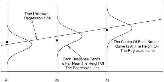
Figure 2.3 illustrates some of the assumptions of the basic linear regression model. The data ((x_1,y_1)), ((x_2,y_2)) and ((x_3,y_3)) are observed and are represented by the circular opaque plotting symbols. According to the model, these observations should be close to the regression line (mathrm{E}~y = beta_0 + beta_1 x). Each deviation from the line is random. We will often assume that the distribution of deviations may be represented by a normal curve, as in Figure 2.3.
R Code for Figure 2.3
The basic linear regression model assumptions describe the underlying population. Table 2.2 highlights the idea that characteristics of this population can be summarized by the parameters (beta_0), (beta_1) and (sigma ^{2}). In Section 2.1, we summarized data from a sample, introducing the statistics (b_0) and (b_1). Section 2.3 will introduce (s^{2}), the statistic corresponding to the parameter (sigma ^{2}).
begin{array}{c}
text{Table 2.2 Summary Measures of the Population and Sample}\
end{array}\
begin{array}{cccc} hline text{Data} & phantom{XXX}text{Summary} & phantom{XX}text{Regression} & text{Variance} \ & phantom{XXX}text{Measures} & phantom{XXX}text{Line} & end{array}\
begin{array}{ccccc}& & text{Intercept} & text{Slope} & \ hline text{Population} & text{Parameters} & beta_0 & beta_1 & sigma ^{2} \ text{Sample} & text{Statistics} & b_0 & b_1 & s^2 \ hline end{array} end{matrix}