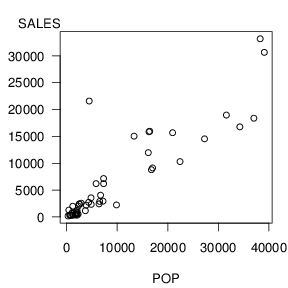
The basic graphical tool used to investigate the relationship between the two variables is a scatter plot such as in Figure 2.2. Although we may lose the exact values of the observations when graphing data, we gain a visual impression of the relationship between population and sales. From Figure 2.2 we see that areas with larger populations tend to purchase more lottery tickets. How strong is this relationship? Can knowledge of the area’s population help us anticipate the revenue from lottery sales? We explore these two questions below.
R Code for Figure 2.2
One way to summarize the strength of the relationship between two variables is through a correlation statistic.
$$r=\frac{1}{(n-1)s_x s_y} \sum_{i=1}^{n}\left( x_{i}-\overline{x} \right) \left( y_{i}- \overline{y} \right) .$$
Here, we use the sample standard deviation $s_y = \sqrt{(n-1)^{-1} \sum_{i=1}^{n} \left( y_i – \overline{y} \right)^{2}}$ defined in Section 1.2, with similar notation for $s_x$.
Although there are other correlation statistics, the correlation coefficient devised by Pearson (1895) has several desirable properties. One important property is that, for any data set, r is bounded by $-1$ and $1$, that is, $-1 \leq r \le 1$. (Exercise 2A.9 provides steps for you to check this property.) If r is greater than zero, the variables are said to be (positively) correlated. If r is less than zero, the variables are said to be negatively correlated. The larger the coefficient is in absolute value, the stronger is the relationship. In fact, if $r=1$, then the variables are perfectly correlated. In this case, all of the data lie on a straight line that goes through the lower left and upper right-hand quadrants. If $r=-1$, then all of the data lie on a line that goes through the upper left and lower right-hand quadrants. The coefficient r is a measure of a linear relationship between two variables.
The correlation coefficient is said to be location and scale invariant. Thus, each variable’s center of location does not matter in the calculation of r. For example, if we add \$100 to the sales of each zip code, each $y_i$ will increase by 100. However, $\overline{y}$, the average purchase price will also increase by 100 so that the deviation $y_i – \overline{y}$ remains unchanged, or invariant. Further, the scale of each variable does not matter in the calculation of $r$. For example, suppose we divide each population by 1000 so that $x_i$ now represents population in thousands. Thus, $\overline{x}$ is also divided by 1000 and you should check that $s_x$ is also divided by 1000. Thus, the standardized version of $x_i$, $\left( x_i-\overline{x} \right) /s_x$, remains unchanged, or invariant. Many statistical packages compute a standardized version of a variable by subtracting the average and dividing by the standard deviation. Now, let’s use $y_{i,std}=\left( y_i- \overline{y} \right) /s_y$ and $x_{i,std} = \left( x_i-\overline{x} \right) /s_x$ to be the standardized versions of $y_i$ and $x_i$, respectively. With this notation, we can express the correlation coefficient as $r=(n-1)^{-1}\sum_{i=1}^{n} x_{i,std} \times y_{i,std}.$
The correlation coefficient is said to be a dimensionless measure. This is because we have taken away dollars, and all other units of measures, by considering the standardized variables $x_{i,std}$ and $y_{i,std}$. Because the correlation coefficient does not depend on units of measure, it is a statistic that can readily be compared across different data sets.
In the world of business, the term “correlation” is often used as synonymous with the term “relationship.” For the purposes of this text, we use the term correlation when referring only to linear relationships. The classic nonlinear relationship is $y=x^{2}$, a quadratic relationship. Consider this relationship and the fictitious data set for x, ({-2,1,0,1,2}). Now, as an exercise, produce a rough graph of the data set:
\begin{matrix}\begin{array}{l|rrrrr} \hline i & 1 & 2 & 3 & 4 & 5 \\ x_i & -2 & -1 & 0 & 1 & 2 \\ y_i & 4 & 1 & 0 & 1 & 4 \\ \hline \end{array} \end{matrix}
The correlation coefficient for this data set turns out to be $r=0$ (check this). Thus, despite the fact that there is a perfect relationship between x and y ($=x^{2}$), there is a zero correlation. Recall that location and scale changes are not relevant in correlation discussions, so we could easily change the values of x and y to be more representative of a business data set.
How strong is the relationship between y and x for the lottery data? Graphically, the response is a scatter plot, as in Figure 2.2. Numerically, the main response is the correlation coefficient which turns out to be r = 0.886 for this data set. We interpret this statistic by saying that SALES and POP are (positively) correlated. The strength of the relationship is strong because r = 0.886 is close to one. In summary, we may describe this relationship by saying that there is a strong correlation between SALES and POP.