3.3.1 Functions of Random Variables and their Distributions

In Section 3.2 we discussed some elementary known distributions. In this section we discuss means of creating new parametric probability distributions from existing ones. Let $X$ be a continuous random variable with a known probability density function $f_{X}(x)$ and distribution function $F_{X}(x)$. Consider the transformation $Y = gleft( X right)$, where $g(X)$ is a one-to-one transformation defining a new random variable $Y$. We can use the distribution function technique, the change-of-variable technique or the moment-generating function technique to find the probability density function of the variable of interest $Y$. In this section we apply the following techniques for creating new families of distributions: (a) multiplication by a constant (b) raising to a power, (c) exponentiation and (d) mixing.

Multiplication by a Constant

If claim data show change over time then such transformation can be useful to adjust for inflation. If the level of inflation is positive then claim costs are rising, and if it is negative then costs are falling. To adjust for inflation we multiply the cost $X$ by 1+ inflation rate (negative inflation is deflation). To account for currency impact on claim costs we also use a transformation to apply currency conversion from a base to a counter currency.

Consider the transformation $Y = cX$, where $c > 0$, then the distribution function of $Y$ is given by
$$F_{Y}left( y right) = Prleft( Y leq y right) = Prleft( cX leq y right) = Prleft( X leq frac{y}{c} right) = F_{X}left( frac{y}{c} right).$$
Hence, the probability density function of interest $f_{Y}(y)$ can be written as
$$f_{Y}left( y right) = frac{1}{c}f_{X}left( frac{y}{c} right).$$
Suppose that $X$ belongs to a certain set of parametric distributions and define a rescaled version $Y = cX$, $c > 0$. If $Y$ is in the same set of distributions then the distribution is said to be a scale distribution. When a member of a scale distribution is multiplied by a constant $c$ ($c > 0$), the scale parameter for this scale distribution meets two conditions:

1. The parameter is changed by multiplying by $c$;
2. All other parameter remain unchanged.

Example 3.7 (SOA) The aggregate losses of Eiffel Auto Insurance are denoted in Euro currency and follow a Lognormal distribution with $mu = 8$ and $sigma = 2$. Given that 1 euro $=$ 1.3 dollars, find the set of lognormal parameters, which describe the distribution of Eiffel’s losses in dollars?
Solution

Example 3.8 Demonstrate that the gamma distribution is a scale distribution.
Solution

Raising to a Power

In the previous section we have talked about the flexibility of the Weibull distribution in fitting reliability data. Looking to the origins of the Weibull distribution, we recognize that the Weibull is a power transformation of the exponential distribution. This is an application of another type of transformation which involves raising the random variable to a power.

Consider the transformation $Y = X^{tau}$, where $tau > 0$, then the distribution function of $Y$ is given by
$$F_{Y}left( y right) = Prleft( Y leq y right) = Prleft( X^{tau} leq y right) = Prleft( X leq y^{1/ tau} right) = F_{X}left( y^{1/ tau} right).$$

Hence, the probability density function of interest $f_{Y}(y)$ can be written as
$$f_{Y}(y) = frac{1}{tau} y^{1/ tau – 1} f_{X}left( y^{1/ tau} right).$$
On the other hand, if $tau lt 0$, then the distribution function of $Y$ is given by
$$F_{Y}left( y right) = Prleft( Y leq y right) = Prleft( X^{tau} leq y right) = Prleft( X geq y^{1/ tau} right) = 1 – F_{X}left( y^{1/ tau} right), $$
and
$$f_{Y}(y) = left| frac{1}{tau} right|{y^{1/ tau – 1}f}_{X}left( y^{1/ tau} right).$$

Example 3.9 We assume that $X$ follows the exponential distribution with mean $theta$ and consider the transformed variable $Y = X^{tau}$. Show that
$Y$ follows the Weibull distribution when $tau$ is positive and determine the parameters of the Weibull distribution.
Solution

Exponentiation

The normal distribution is a very popular model for a wide number of applications and when the sample size is large, it can serve as an approximate distribution for other models. If the random variable $X$ has a normal distribution with mean $mu$ and variance $sigma^{2}$, then $Y = e^{X}$ has lognormal distribution with parameters $mu$ and $sigma^{2}$. The lognormal random variable has a lower bound of zero, is positively skewed and has a long right tail. A lognormal distribution is commonly used to describe distributions of financial assets such as stock prices. It is also used in fitting claim amounts for automobile as well as health insurance. This is an example of another type of transformation which involves exponentiation.

Consider the transformation $Y = e^{X}$, then the distribution function of $Y$ is given by
$$F_{Y}left( y right) = Prleft( Y leq y right) = Prleft( e^{X} leq y right) = Prleft( X leq ln y right) = F_{X}left( ln y right).$$
Hence, the probability density function of interest $f_{Y}(y)$ can be written as
$$f_{Y}(y) = frac{1}{y}f_{X}left( ln y right).$$

Example 3.10 (SOA) $X$ has a uniform distribution on the interval $(0, c)$. $Y = e^{X}$. Find the distribution of $Y$.
Solution

3.3.2 Finite Mixtures

Mixture distributions represent a useful way of modelling data that are drawn from a heterogeneous population. This parent population can be
thought to be divided into multiple subpopulations with distinct distributions.

Two-point mixture

If the underlying phenomenon is diverse and can actually be described as two phenomena representing two subpopulations with different modes, we can construct the two point mixture random variable $X$. Given random variables $X_{1}$ and $X_{2}$, with probability density functions $f_{X_{1}}left( x right)$ and $f_{X_{2}}left( x right)$ respectively, the probability density function of $X$ is the weighted average of the component probability density function $f_{X_{1}}left( x right)$ and $f_{X_{2}}left( x right)$. The probability density function and distribution function of $X$ are given by
$$f_{X}left( x right) = af_{X_{1}}left( x right) + left( 1 – a right)f_{X_{2}}left( x right),$$
and
$$F_{X}left( x right) = aF_{X_{1}}left( x right) + left( 1 – a right)F_{X_{2}}left( x right),$$

for $0 lt a lt 1$, where the mixing parameters $a$ and $(1 – a)$ represent the proportions of data points that fall under each of the two subpopulations respectively. This weighted average can be applied to a number of other distribution related quantities. The k-th moment and moment generating function of $X$ are given by
$Eleft( X^{k} right) = aEleft( X_{1}^{K} right) + left( 1 – a right)Eleft( X_{2}^{k} right)$,
and
$$M_{X}left( t right) = aM_{X_{1}}left( t right) + left( 1 – a right)M_{X_{2}}left( t right),$$ respectively.

Example 3.11 (SOA) The distribution of the random variable $X$ is an equally weighted mixture of two Poisson distributions with parameters $lambda_{1}$ and $lambda_{2}$ respectively. The mean and variance of $X$ are 4 and 13, respectively. Determine $Prleft( X > 2 right)$.
Solution

k-point mixture

In case of finite mixture distributions, the random variable of interest $X$ has a probability $p_{i}$ of being drawn from homogeneous subpopulation $i$, where $i = 1,2,ldots,k$ and $k$ is the initially specified number of subpopulations in our mixture. The mixing parameter $p_{i}$ represents the proportion of observations from subpopulation $i$. Consider the random variable $X$ generated from $k$ distinct subpopulations, where subpopulation $i$ is modeled by the continuous distribution $f_{X_{i}}left( x right)$. The probability distribution of $X$ is given by
$$f_{X}left( x right) = sum_{i = 1}^{k}{p_{i}f_{X_{i}}left( x right)},$$
where $0 lt p_{i} lt 1$ and $sum_{i = 1}^{k} p_{i} = 1$.

This model is often referred to as a finite mixture or a $k$ point mixture. The distribution function, $r$-th moment and moment generating functions of the $k$-th point mixture are given as

$$F_{X}left( x right) = sum_{i = 1}^{k}{p_{i}F_{X_{i}}left( x right)},$$
$$Eleft( X^{r} right) = sum_{i = 1}^{k}{p_{i}Eleft( X_{i}^{r} right)}, text{and}$$
$$M_{X}left( t right) = sum_{i = 1}^{k}{p_{i}M_{X_{i}}left( t right)},$$ respectively.

Example 3.12 (SOA) $Y_{1}$ is a mixture of $X_{1}$ and $X_{2}$ with mixing weights $a$ and $(1 – a)$. $Y_{2}$ is a mixture of $X_{3}$ and $X_{4}$ with mixing weights $b$ and $(1 – b)$. $Z$ is a mixture of $Y_{1}$ and $Y_{2}$ with mixing weights $c$ and $(1 – c)$.

Show that $Z$ is a mixture of $X_{1}$, $X_{2}$, $X_{3}$ and $X_{4}$, and find the mixing weights.
Solution

3.3.3 Continuous Mixtures

A mixture with a very large number of subpopulations ($k$ goes to infinity) is often referred to as a continuous mixture. In a continuous mixture, subpopulations are not distinguished by a discrete mixing parameter but by a continuous variable $theta$, where $theta$ plays the role of $p_{i}$ in the finite mixture. Consider the random variable $X$ with a distribution depending on a parameter $theta$, where $theta$ itself is a continuous random variable. This description yields the following model for $X$
$$f_{X}left( x right) = int_{0}^{infty}{f_{X}left( xleft| theta right. right)gleft( theta right)} d theta ,$$ where $f_{X}left( xleft| theta right. right)$ is the conditional distribution of $X$ at a particular value of $theta$ and $gleft( theta right)$ is the probability statement made about the unknown parameter $theta$, known as the prior distribution of $theta$ (the prior information or expert opinion to be used in the analysis).

The distribution function, $k$-th moment and moment generating functions of the continuous mixture are given as
$$F_{X}left( x right) = int_{-infty}^{infty}{F_{X}left( xleft| theta right. right)gleft( theta right)} d theta,$$
$$Eleft( X^{k} right) = int_{-infty}^{infty}{Eleft( X^{k}left| theta right. right)gleft( theta right)}d theta,$$
$$M_{X}left( t right) = Eleft( e^{t X} right) = int_{-infty}^{infty}{Eleft( e^{ tx}left| theta right. right)gleft( theta right)}d theta, $$ respectively.

The $k$-th moments of the mixture distribution can be rewritten as
$$Eleft( X^{k} right) = int_{-infty}^{infty}{Eleft( X^{k}left| theta right. right)gleft( theta right)}dtheta = Eleftlbrack Eleft( X^{k}left| theta right. right) rightrbrack .$$

In particular the mean and variance of $X$ are given by
$$Eleft( X right) = Eleftlbrack Eleft( Xleft| theta right. right) rightrbrack$$
and
$$Varleft( X right) = Eleftlbrack Varleft( Xleft| theta right. right) rightrbrack + Varleftlbrack Eleft( Xleft| theta right. right) rightrbrack .$$

Example 3.13 (SOA) $X$ has a binomial distribution with a mean of $100q$ and a variance of $100qleft( 1 – q right)$ and $q$ has a beta distribution with parameters $a = 3$ and $b = 2$. Find the unconditional mean and variance of $X$.
Solution

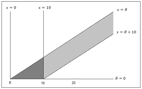
Exercise 3.14 (SOA) Claim sizes, $X$, are uniform on for each policyholder. varies by policyholder according to an exponential distribution with mean 5. Find the unconditional distribution, mean and variance of $X$.
Solution