The Gamma Distribution
The gamma distribution is commonly used in modeling claim severity. The traditional approach in modelling losses is to fit separate models for claim frequency and claim severity. When frequency and severity are modeled separately it is common for actuaries to use the Poisson distribution for claim count and the gamma distribution to model severity. An alternative approach for modelling losses that has recently gained popularity is to create a single model for pure premium (average claim cost) that will be described in Chapter 4.
The continuous variable $X$ is said to have the gamma distribution with shape parameter $alpha$ and scale parameter $theta$ if its probability
density function is given by
$$f_{X}left( x right) = frac{left( x/ theta right)^{alpha}}{xGammaleft( alpha right)}exp left( -x/ theta right) text{for } x gt 0 .$$
Note that $ alpha gt 0, theta gt 0$.
Figures 3.1 and 3.2 demonstrate the effect of the shape and scale parameters on the gamma density function.
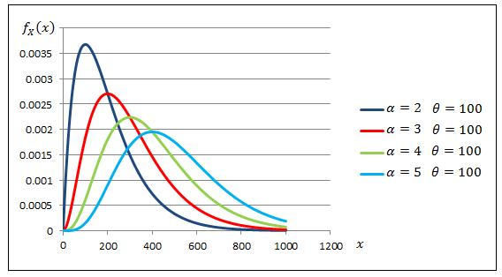
Fig. 3.1. Gamma Density Functions with Varying Scale Parameters
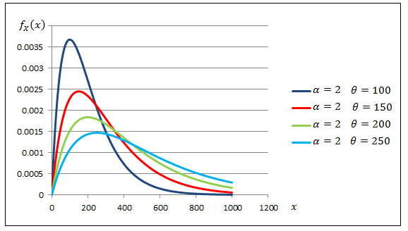
Fig. 3.2 Gamma Density Functions with Varying Shape Parameters
When $alpha = 1$ the gamma reduces to an exponential distribution and when $alpha = frac{n}{2}$ and $theta = 2$ the gamma reduces to a chi-square distribution with $n$ degrees of freedom. As we will see in Section 3.6.2, the chi-square distribution is used extensively in statistical hypothesis testing.
The distribution function of the gamma model is the incomplete gamma function, denoted by $Gammaleft( frac{alpha;x}{theta} right)$, and defined as
$$F_{X}left( x right) = Gammaleft( alpha; frac{x}{theta} right) = frac{1}{Gammaleft( alpha right)}int_{0}^{x /theta}t^{alpha – 1}e^{- t}text{dt}$$
$alpha gt 0, theta gt 0$.
The $k$-th moment of the gamma distributed random variable for any positive $k$ is given by
$$Eleft( X^{k} right) = theta^{k} frac{Gammaleft( alpha + k right)}{Gammaleft( alpha right)} text{for } k gt 0 .$$
The mean and variance are given by $Eleft( X right) = alphatheta$ and $Varleft( X right) = alphatheta^{2}$, respectively.
Since all moments exist for any positive $k$, the gamma distribution is considered a light tailed distribution, which may not be suitable for
modeling risky assets as it will not provide a realistic assessment of the likelihood of severe losses.
The Pareto Distribution
The Pareto distribution, named after the Italian economist Vilfredo Pareto (1843–1923), has many economic and financial applications. It is a positively skewed and heavy-tailed distribution which makes it suitable for modeling income, high-risk insurance claims and severity of large casualty losses. The survival function of the Pareto distribution which decays slowly to zero was first used to describe the distribution of income where a small percentage of the population holds a large proportion of the total wealth. For extreme insurance claims, the tail of the severity distribution (losses in excess of a threshold) can be modelled using a Pareto distribution.
The continuous variable $X$ is said to have the Pareto distribution with shape parameter $alpha$ and scale parameter $theta$ if its pdf is given by
$$f_{X}left( x right) = frac{alphatheta^{alpha}}{left( x + theta right)^{alpha + 1}} x gt 0, alpha gt 0, theta gt 0.$$
Figures 3.3 and 3.4 demonstrate the effect of the shape and scale parameters on the Pareto density function.
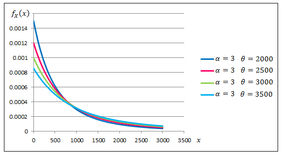
Fig. 3.3. Pareto Density Functions with Varying Scale Parameters
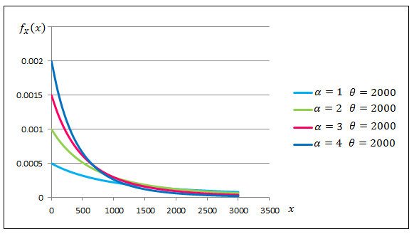
Fig. 3.4. Pareto Density Functions with Varying Shape Parameters
The distribution function of the Pareto distribution is given by
$$F_{X}left( x right) = 1 – left( frac{theta}{x + theta} right)^{alpha} x gt 0, alpha gt 0, theta gt 0.$$
It can be easily seen that the hazard function of the Pareto distribution is a decreasing function in $x$, another indication that the distribution is heavy tailed.
The $k$-th moment of the Pareto distributed random variable exists, if and only if, $alpha gt k$. If $k$ is a positive integer then
$$Eleft( X^{k} right) = frac{k!theta^{k}}{left( alpha – 1 right)cdotsleft( alpha – k right)} alpha gt k.$$
The mean and variance are given by $$Eleft( X right) = frac{theta}{alpha – 1} text{for } alpha gt 1$$ and
$$Varleft( X right) = frac{alphatheta^{2}}{left( alpha – 1 right)^{2}left( alpha – 2 right)} text{for } alpha gt 2,$$respectively.
Example 3.5 The claim size of an insurance portfolio follows the Pareto distribution with mean and variance of 40 and 1800 respectively. Find
- The shape and scale parameters.
- The 95-th percentile of this distribution.
The Weibull Distribution
The Weibull distribution, named after the Swedish physicist Waloddi Weibull (1887-1979) is widely used in reliability, life data analysis, weather forecasts and general insurance claims. Truncated data arise frequently in insurance studies. The Weibull distribution is particularly useful in modeling left-truncated claim severity distributions. Weibull was used to model excess of loss treaty over automobile insurance as well as earthquake inter-arrival times.
The continuous variable $X$ is said to have the Weibull distribution with shape parameter $alpha$ and scale parameter $theta$ if its probability density function is given by
$$f_{X}left( x right) = frac{alpha}{theta}left( frac{x}{theta} right)^{alpha – 1} exp left(- left( frac{x}{theta} right)^{alpha}right) x gt 0, alpha gt 0, theta gt 0.$$
Figures 3.5 and 3.6 demonstrate the effects of the shape and scale parameters on the Weibull density function.
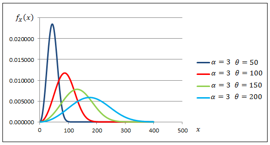
Fig. 3.5 Weibull Density Functions with Varying Scale Parameters
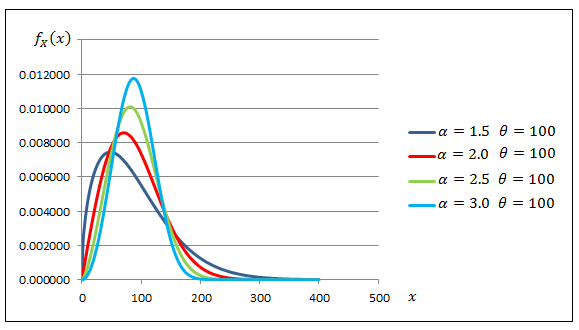
Fig. 3.6 Weibull Density Functions with Varying Shape Parameters
The distribution function of the Weibull distribution is given by
$$F_{X}left( x right) = 1 – e^{- left( x / theta right)^{alpha}} x gt 0, alpha gt 0, theta gt 0.$$
It can be easily seen that the shape parameter $alpha$ describes the shape of the hazard function of the Weibull distribution. The hazard function is a decreasing function when $alpha lt 1$, constant when $alpha = 1$ and increasing when $alpha gt 1$. This behavior of the hazard function makes the Weibull distribution a suitable model for a wide variety of phenomena such as weather forecasting, electrical and industrial engineering, insurance modeling and financial risk analysis.
The $k$-th moment of the Weibull distributed random variable is given by
$$Eleft( X^{k} right) = theta^{k}Gammaleft( 1 + frac{k}{alpha} right) .$$
The mean and variance are given by
$$Eleft( X right) = thetaGammaleft( 1 + frac{1}{alpha} right)$$ and
$$Var(X)= theta^{2}left( Gammaleft( 1 + frac{2}{alpha} right) – leftlbrack Gammaleft( 1 + frac{1}{alpha} right) rightrbrack ^{2}right),$$ respectively.
Example 3.6 Suppose that the probability distribution of the lifetime of AIDS patients (in months) from the time of diagnosis is described by the Weibull distribution with shape parameter 1.2 and scale parameter 33.33.
- Find the probability that a randomly selected person from this population survives at least 12 months,
- A random sample of 10 patients will be selected from this population. What is the probability that at most two will die within
one year of diagnosis. - Find the 99-th percentile of this distribution.
The Generalized Beta Distribution of the Second Kind
The Generalized Beta Distribution of the Second Kind (GB2) was introduced by Gary Venter (1983) in the context of insurance loss modeling and by MacDonald (1984) as an income and wealth distribution. It is a four-parameter very flexible distribution that can model positively as well as negatively skewed distributions.
The continuous variable $X$ is said to have the GB2 distribution with parameters $a$, $b$, $alpha$ and $beta$ if its probability density function is given by
$$f_{X}left( x right) = frac{ax^{a alpha – 1}}{b^{a alpha}Bleft( alpha,beta right)leftlbrack 1 + left( x/b right)^{a} rightrbrack^{alpha + beta}} text{for } x gt 0,$$
$a,b,alpha,beta gt 0$, and where the beta function $Bleft( alpha,beta right)$ is defined as
$$Bleft( alpha,beta right) = int_{0}^{1}{t^{alpha – 1}left( 1 – t right)^{beta – 1}}text{dt}.$$
The GB2 provides a model for heavy as well as light tailed data. It includes the exponential, gamma, Weibull, Burr, Lomax, F, chi-square, Rayleigh, lognormal and log-logistic as special or limiting cases. For example, by setting the parameters $a = alpha = beta = 1$, then the GB2 reduces to the log-logistic distribution. When $a = 1$ and $beta rightarrow infty$, it reduces to the gamma distribution and when $alpha = 1$ and $beta rightarrow infty$, it reduces to the Weibull distribution.
The $k$-th moment of the GB2 distributed random variable is given by
$$Eleft( X^{k} right) = frac{b^{k}left( alpha + frac{k}{a},beta – frac{k}{a} right)}{left( alpha,beta right)}, k gt 0.$$
Earlier applications of the GB2 were on income data and more recently have been used to model long-tailed claims data. GB2 was used to model different types of automobile insurance claims, severity of fire losses as well as medical insurance claim data.