With Monte Carlo, or stochastic, simulation, we get additional insights. To illustrate ideas, we focus on the loss random variable at (t=10).
Let (U) be a randomly generated uniform random number on ((0,1)). In this case, the future (given (T>10)) remaining lifetime random variable (T -10 = 55*U), that is, uniform on the interval ((0,55)). For this randomly generated future lifetime, the corresponding loss random variable is
begin{eqnarray*}
L_t^n = v^{T-10} – 0.020266~ bar{a}_{overline{T-10}|}.
end{eqnarray*}
We generated 100,000 replications of this loss random variable (taking less than two seconds on a moderately slow notebook). Figure 3 summarizes the distribution of these replications. The average of this distribution turned out to be 0.055512; this is very close to the theoretically correct value determined above, 0.055701. The standard deviation from the Figure 3 sample is 0.3459959, close to 0.3466074 that was determined by theory. Figure 3 shows that the maximum value is 1.0 (corresponding to (T=10)) and the minimum value is -0.29310, corresponding to (T=65).
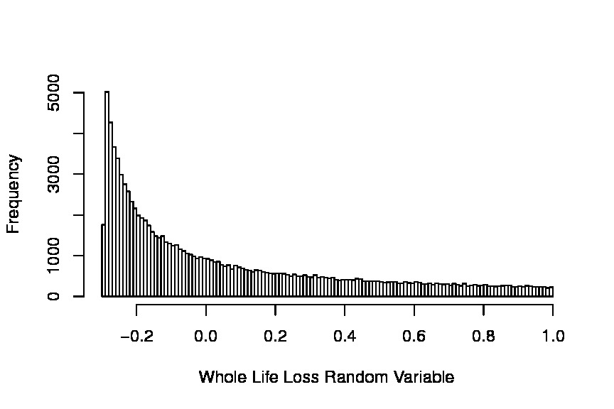
The simulation gives a quick method to calculate the same values that we could determine from theory. Simulation also allows us to readily see the entire distribution of the loss random variable – for this simple example, we could determine the distribution from theory. Moreover, theoretical calculations allow us to readily visualize patterns over evolving time duration (t). As we will see, the advantage of simulation methods is that they provide flexibility to easily modify design aspects such as timing of benefits and payments, as well as for discounting mechanisms such as variable interest rates. You will find it helpful to become facile in doing calculations using both theory and simulation approaches.
Try an animated display where the distribution changes by the policy duration