Mixed Distribution Example. Consider a random variable that is 0 with probability 70% and is exponentially distributed with parameter (theta= 10,000) with probability 30%. In practice, this might correspond to a 70% chance of having no insurance claims and a 30% chance of a claim – if a claim occurs, then it is exponentially distributed. The distribution function is given as
begin{eqnarray*}
F(y) = left{ begin{array}{cc}
0 & x <0 \
1 - 0.3 exp(-x/10000) & x ge 0 .
end{array} right.
end{eqnarray*}
Figure 3. Mixed Distribution Function
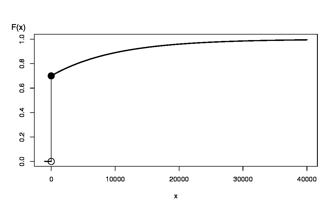
From the graph, we can see that the inverse transform for generating random variables with this distribution function is
begin{eqnarray*}
X = F^{-1}(U) = left{
begin{array}{cc}
0 & 0< U< 0.7 \
-1000 ln left(frac{1-U}{0.3}right) & 0.7 le U < 1 .
end{array} right.
end{eqnarray*}
As you have seen, for the discrete and mixed random variables, the key is to draw a graph of the distribution function. This allows you to visualize potential values of the inverse function.
[previous][next]