Discrete Distribution Example. Consider the time of a machine failure in the first five years. The distribution of failure times is given as:
| Time ((x)) | 1 | 2 | 3 | 4 | 5 |
| Probability | 0.1 | 0.2 | 0.1 | 0.4 | 0.2 |
| (F(x)) | 0.1 | 0.3 | 0.4 | 0.8 |
Figure 2. Discrete Distribution Function
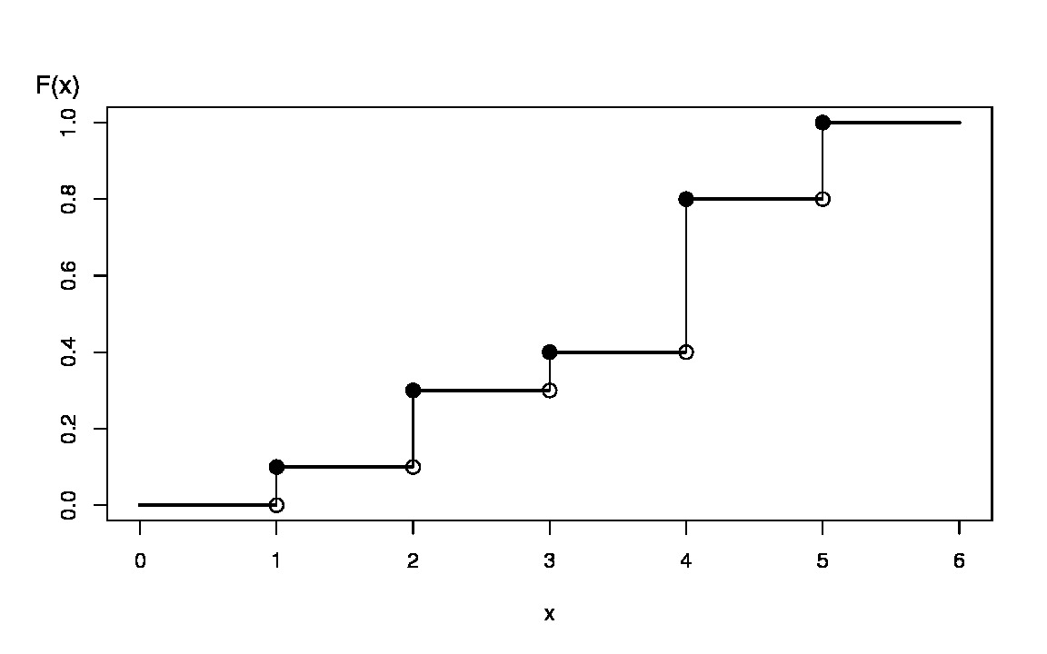
Using the graph of the distribution function, with the inverse transform we may define
begin{eqnarray*}
X = left{ begin{array}{cc}
1 & 0 lt U lt 0.1 \
2 & 0.1 leq U lt 0.3\
3 & 0.3 leq U lt 0.4\
4 & 0.4 leq U lt 0.8 \
5 & 0.8 leq U lt 1.0 .
end{array} right.
end{eqnarray*}
For general discrete random variables, there may not be an ordering of outcomes. For example, a person could own one of five types of life insurance products and we might use the following algorithm to generate random outcomes:
begin{eqnarray*}
X = left{ begin{array}{cc}
textrm{whole life} & 0 < U < 0.1 \
textrm{endowment} & 0.1 leq U < 0.3\
textrm{term life} & 0.3 leq U < 0.4\
textrm{universal life} & 0.4 leq U < 0.8 \
textrm{variable life} & 0.8 leq U < 1.0 .
end{array} right.
end{eqnarray*}
Another analyst may use an alternative procedure such as:
begin{eqnarray*}
X = left{
begin{array}{cc}
textrm{whole life} & 0.9 < U < 1.0 \
textrm{endowment} & 0.7 leq U < 0.9\
textrm{term life} & 0.6 leq U < 0.7\
textrm{universal life} & 0.2 leq U < 0.6 \
textrm{variable life} & 0 leq U < 0.2 .
end{array} right.
end{eqnarray*}
Both algorithms produce (in the long-run) the same probabilities, e.g., (Pr(textrm{whole life})=0.1), and so forth. So, neither is incorrect. You should be aware that there is "more than one way to skin a cat." (What an old expression!) Similarly, you could use an alternative algorithm for ordered outcomes (such as failure times 1, 2, 3, 4, or 5, above).
[previous][next]