Introduction
Stata notes
This workshop series assumes you already have a knowledge of Structural Equation Modeling, and are mainly interested in learning how to use Stata to estimate these models. We will start with simple models, and try to make things more complicated/nuanced from there.
There are two core Stata commands for structural equation modeling: sem for models built on multivariate normal assumptions, and gsem for models with generalized linear components.
In the usual Stata command style, both sem and gsem will be used as estimation commands, and each will allow a host of post-estimation commands to further examine the models.
We will take our first example from the MPlus documentation.
infile x1-x3 using "..\..\MPlus\Basics\Sample stats\ex3.1.dat"
* The file is found at
*    "http://www.ssc.wisc.edu/~hemken/MPlus/Basics/Sample stats/ex3.1.dat"
(500 observations read)
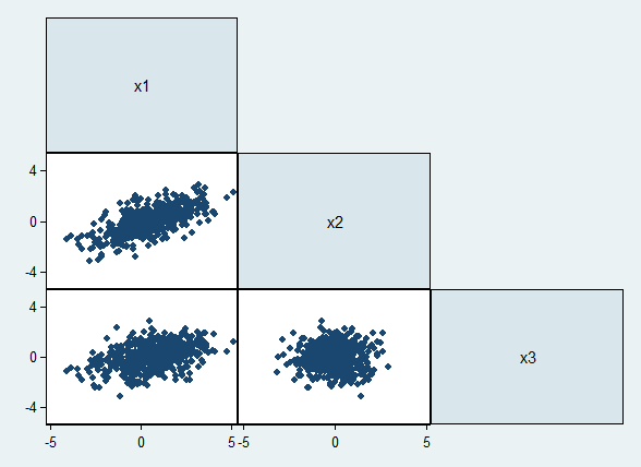
A quick visualization of our data shows us three variables with differing degrees of correlation:
graph matrix _all, half maxes(yscale(range(-5 5)) ylabel(-4(4)4))
We can start by using the usual Stata commands to look at some descriptive statistics for our data. One of the advantages of using Stata for SEM is that we have all of the usual data manipulation and statistical commands at our fingertips!
correlate , means covariance
    Variable |         Mean    Std. Dev.          Min          Max
-------------+----------------------------------------------------
          x1 |     .4848463     1.553196    -4.116261     5.111009
          x2 |      .001289     1.046764    -3.145148      2.92044
          x3 |    -.0421612     .9791309    -3.138746     2.875135

             |       x1       x2       x3
-------------+---------------------------
          x1 |  2.41242
          x2 |  1.08062  1.09571
          x3 |   .64962  .028249  .958697
These are sample covariances, with \(N-1\) used in the denominator. Stata's sem command reports maximum likelihood covariances, with \(N\) used in the denominator. We can use the usual Stata command language to convert like this:
matrix CV = r(C)*(r(N)-1)/r(N)
matrix list CV
symmetric CV[3,3]
           x1         x2         x3
x1  2.4075922
x2  1.0784573  1.0935232
x3  .64832035  .02819297  .95677985
Covariance Model
The covariances (plus the means) form a saturated model for our data, that is, they perfectly fit the covariance matrix (plus the means vector).
(Check this against the previous result.)
sem (x1-x3 -> )
Exogenous variables

Observed:  x1 x2 x3

Fitting target model:

Iteration 0:   log likelihood =  -2124.388
Iteration 1:   log likelihood =  -2124.388

Structural equation model                       Number of obs     =        500
Estimation method  = ml
Log likelihood     =  -2124.388

------------------------------------------------------------------------------
             |                 OIM
             |      Coef.   Std. Err.      z    P>|z|     [95% Conf. Interval]
-------------+----------------------------------------------------------------
     mean(x1)|   .4848463   .0693915     6.99   0.000     .3488414    .6208512
     mean(x2)|    .001289   .0467659     0.03   0.978    -.0903704    .0929484
     mean(x3)|  -.0421612   .0437443    -0.96   0.335    -.1278984    .0435759
-------------+----------------------------------------------------------------
      var(x1)|   2.407592   .1522695                      2.126906    2.725321
      var(x2)|   1.093523   .0691605                       .966036    1.237835
      var(x3)|   .9567799   .0605121                      .8452347    1.083046
-------------+----------------------------------------------------------------
   cov(x1,x2)|   1.078457   .0871301    12.38   0.000     .9076854    1.249229
   cov(x1,x3)|   .6483204   .0738086     8.78   0.000     .5036581    .7929826
   cov(x2,x3)|    .028193   .0457615     0.62   0.538    -.0614979    .1178838
------------------------------------------------------------------------------
LR test of model vs. saturated: chi2(0)   =      0.00, Prob > chi2 =      .
Model Specification
Paths are specified in sem using parentheses and an "arrow", which may point either to the left or to the right (-> or <- are equivalent).
Multiple variables (we may use Stata`s typical varlist shortcuts) may be collected on either side of the path arrow, or paths may be specified separately. Our covariance model could be written
sem (x1-x3 -> )
sem (<- x1-x3 )
sem (x1->)(<-x2)(x3->)
(You ought to be able to come up with a few more variants.)
Sample Covariances, instead
Alternatively, we can have sem report sample covariances:
sem (x1-x3 -> ), nm1 // sample covariances instead of ML
Exogenous variables

Observed:  x1 x2 x3

Fitting target model:

Iteration 0:   log likelihood = -2125.8895
Iteration 1:   log likelihood = -2125.8895

Structural equation model                       Number of obs     =        500
Estimation method  = ml
Log likelihood     = -2125.8895

------------------------------------------------------------------------------
             |                 OIM
             |      Coef.   Std. Err.      z    P>|z|     [95% Conf. Interval]
-------------+----------------------------------------------------------------
     mean(x1)|   .4848463    .069461     6.98   0.000     .3487052    .6209874
     mean(x2)|    .001289   .0468127     0.03   0.978    -.0904622    .0930402
     mean(x3)|  -.0421612   .0437881    -0.96   0.336    -.1279843    .0436618
-------------+----------------------------------------------------------------
      var(x1)|   2.412417   .1525746                      2.131168    2.730782
      var(x2)|   1.095715   .0692991                      .9679719    1.240316
      var(x3)|   .9586972   .0606333                      .8469285    1.085216
-------------+----------------------------------------------------------------
   cov(x1,x2)|   1.080619   .0873047    12.38   0.000     .9095044    1.251733
   cov(x1,x3)|   .6496196   .0739565     8.78   0.000     .5046675    .7945717
   cov(x2,x3)|   .0282495   .0458532     0.62   0.538    -.0616211      .11812
------------------------------------------------------------------------------
LR test of model vs. saturated: chi2(0)   =      0.00, Prob > chi2 =      .
Correlations
If we are interested in the standardized solution to this model, this would be just the correlation matrix.
correlate
pwcorr, sig
sem (x1-x3 -> ), standardized
             |       x1       x2       x3
-------------+---------------------------
          x1 |   1.0000
          x2 |   0.6647   1.0000
          x3 |   0.4272   0.0276   1.0000

             |       x1       x2       x3
-------------+---------------------------
          x1 |   1.0000
             |
             |
          x2 |   0.6647   1.0000
             |   0.0000
             |
          x3 |   0.4272   0.0276   1.0000
             |   0.0000   0.5386
             |


Exogenous variables

Observed:  x1 x2 x3

Fitting target model:

Iteration 0:   log likelihood =  -2124.388
Iteration 1:   log likelihood =  -2124.388

Structural equation model                       Number of obs     =        500
Estimation method  = ml
Log likelihood     =  -2124.388

------------------------------------------------------------------------------
             |                 OIM
Standardized |      Coef.   Std. Err.      z    P>|z|     [95% Conf. Interval]
-------------+----------------------------------------------------------------
     mean(x1)|   .3124731      .0458     6.82   0.000     .2227067    .4022394
     mean(x2)|   .0012327   .0447214     0.03   0.978    -.0864196    .0888849
     mean(x3)|   -.043103   .0447421    -0.96   0.335    -.1307959      .04459
-------------+----------------------------------------------------------------
      var(x1)|          1          .                             .           .
      var(x2)|          1          .                             .           .
      var(x3)|          1          .                             .           .
-------------+----------------------------------------------------------------
   cov(x1,x2)|   .6646569   .0249649    26.62   0.000     .6157266    .7135871
   cov(x1,x3)|   .4271616   .0365612    11.68   0.000      .355503    .4988202
   cov(x2,x3)|   .0275626   .0446874     0.62   0.537     -.060023    .1151483
------------------------------------------------------------------------------
LR test of model vs. saturated: chi2(0)   =      0.00, Prob > chi2 =      .
Next: Elementary path models