Data Sources
In Stata, data comes in a variety of forms: the working data set, but also matrices, scalars, and the lists of data objects called "stored results" returned by commands (return and ereturn results).
Data set
Most of the fundamental graphing commands in Stata require data from the working data set. As with statistical analysis in Stata, all of the data required for a graphing problem will generally have to be in just one data set. Depending on the graphing task at hand, you may have to calculate new variables, merge data, reshape data, or calculate summary statistics - in short, any data manipulation task may be part of your set up for graphing.
Keep in mind that the observations in a data set can represent a variety of things. A particularly important distinction for graphing is that some data sets may contain observations of individual units, while other data sets may contain summary statistics for groups of data. For graphing, it is not unusual for a summary data set to be a useful data source.
For example, the following two graph commands use variables from a Stata data set, but while scatter uses individual units of observation, a dot plot of percents within groups uses collapsed data and requires some manipulation to set up.
sysuse autograph twoway scatter mpg weight
preserve
collapse foreign, by(rep78)
replace foreign = foreign *100
label variable foreign "Foreign (%)"
graph dot (asis) foreign, over(rep78)
restoreFrom individual observations:
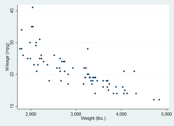
Individual data
From grouped/summary data:
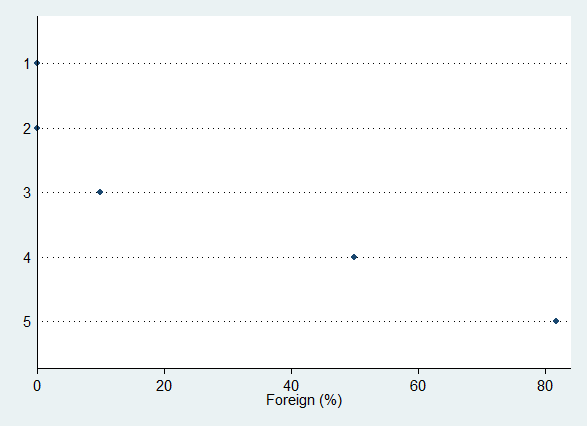
Summary data
Mathematical Scalars and Macro Variables
Not every graphic command requires a data set! In particular it is possible to draw graphs of mathematically specified functions using the twoway function command.
preserve
clear // no data!
graph twoway function y = sqrt(x), range(0 5) ///
    title("{&function}(x) = {&sqrt}x")
restore
Given a function specified in terms of place-holder variables \(y\) and \(x\), and given a data range, Stata draws something akin to a line graph, but without the data. This does require you to specify at least two numerical values, the minimum and the maximum of the graphing range.
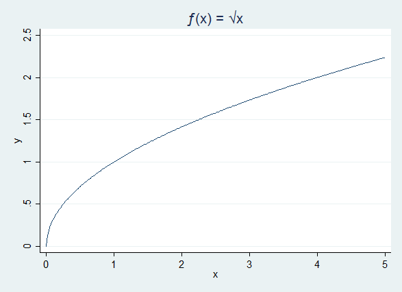
Function graph
At times we may want to draw a graph based on scalar values estimated from our data. An important programming detail is that Stata does not allow us to use Stata’s scalar values in writing code - such numbers have to be converted to macro variables to be sensible to the Stata interpreter.
Suppose we wanted to draw a regression line using twoway function (as we will soon see, we might also use twoway lfit). We need four numerical scalars: the regression slope, the intercept, and a graphing minimum and maximum for \(x\).
quietly summarize weight
local min = r(min) // convert from scalar to macro variable
local max = r(max)
quietly regress mpg weight
local intercept = _b[_cons]
local slope = _b[weight]
* We could clear the data at this point!
twoway function y = `intercept' + `slope'*x, range(`min' `max') ///
    title("Regression line") ytitle("Mileage (mpg)") ///
    xtitle("Weight (lbs.)")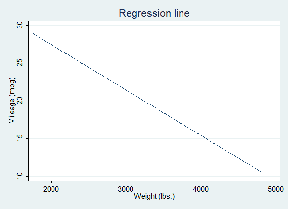
Using macros
In a similar vein, Stata has several "immediate" graphing commands that take numerical arguments: twoway scatteri, twoway pci, and twoway pcarrowi. While these can be used with no data set, they are most often useful to add graphical elements to another graph.
twoway pci 1 1 2 2 ///
    2 2 1 3 ///
    1 3 1 1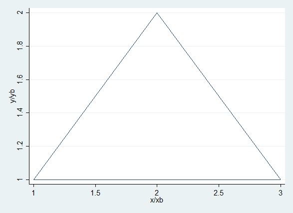
Immediate commands
Stored Results (ereturn)
Finally, there are a number of graphics commands that require you to first estimate something. For example, after a regression you might want to visually examine the distribution of the residuals versus the predicted (fitted) values.
quietly regress mpg c.weight##c.weight
rvfplot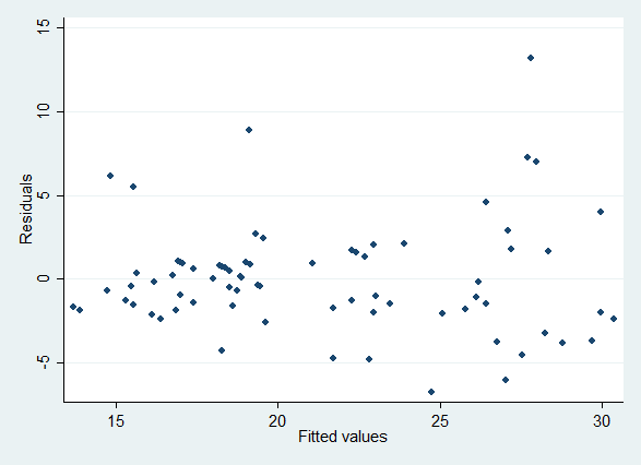
Post-estimation graph