Graphical Elements

At a basic level these are just things like points, line segments, or bounded areas (like polygons). More complicated graphical objects can be constructed out of these basic elements. Stata's graph command will make it easy to specify simple elements as well as treating more complicated objects as fundamental - objects like histograms and boxplots.

Link to Data

The graphs we will consider in Stata are all two-dimensional representations of data. Sometimes elements like points are just positioned in the graph by Cartesian coordinates given by the data values themselves, but other times a point might be given its position by some summary of the data like a group mean. So it can be useful to distinguish between the data set, and the graph-data set. For things like simple scatter plots, these will be one-and-the-same.

Scales (Level of Measurement)

In order to position graphical elements on a page or screen we need some sort of coordinate system. This mainly means Cartesian coordinates. However, Stata will also allow us to distinguish between continuous (Cartesian) scales and categorical scales. Again, this sounds a little abstract, but in practice it is pretty easy.

Some Examples

All of this will be a little more concrete if we look at some examples. We'll start by setting up a familiar data set, auto.

sysuse auto, clear
* Create a categorical variable
generate maker = substr(make, 1, strpos(make, " ")-1)
replace maker = make if strpos(make, " ")==0
label variable maker "Manufacturer"

Consider two graphs. Both use points (dots) as graphical elements to visually represent the data.

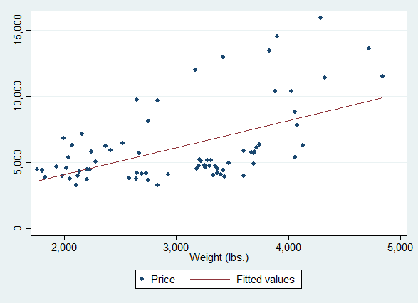
graph twoway scatter price weight
* scatter price weight // abbreviated version
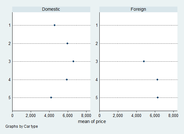
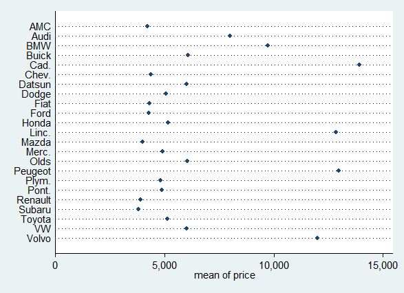
graph dot price, over(maker)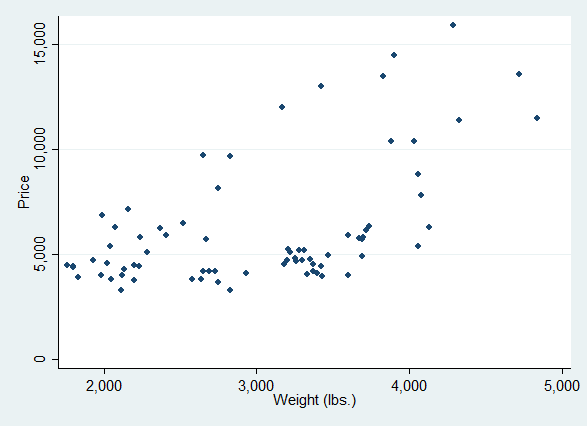

Scatter plot

Here the graphical elements are the points. The position of each point is determined by a pair of data values, the car weight value and the car price value. These data values are used "as is", as they occur in the data set, untransformed. The number of points is (in principle) the same as the number of observations. Both the x- and the y-values are plotted along continuous scales.

Dot plot

In this second graph, the graphical elements are again points. However the vertical position of each point is given by a distinct category, the car maker. The horizontal position of each point is given by a summary statistic, the mean of the prices of cars from a given maker. The number of points is the number of car makers, not the number of observations. The x-values are on a continuous scale, while the y-values are on a categorical scale (as we will see later, Stata switches the "x-" and "y-" nomenclature).

In order to plot the points, the software generates a graph data set (which we never actually see).

Exercises

Use help graph to find commands you may need.

1. Create a bar chart of price versus auto maker. What type of scales are used? Is the height of each bar given by a data value or derived from the data? Use Help to make a second graph where the bars are horizontal.
2. Create a scatterplot matrix of price, weight, and mpg. How many points are shown?
3. Create a boxplot of mpg (gas mileage) versus rep78 (repair record, a Likert scale). What kind of scales are used for graphing? Although each "box" is treated as a fundamental graphical object, it's relation to the data is a little complicated. How are the mid-line, the length of the box, and the length of the whiskers related to the data: data values or derived statistics? The points that appear above one of the boxes?
4. Make a vertical dot plot of price versus rep78. Then make a scatter plot of price versus rep78. How are they similar and how are they different (graphical elements, data, scales)? Why might you prefer one or the other?
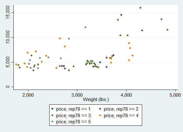
5. Bonus. Continuing from exercise (4), you cannot simply overlay a dot plot and a scatter plot, but just a little data manipulation would allow you to create a visual combination of the two. Do it! (Hint: if you are stuck, come back to this after reading the next section.)
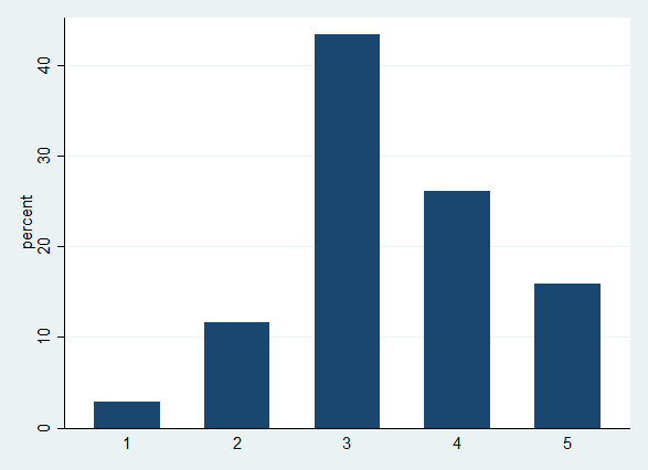
6. Bonus. Histograms are a little more complicated than one might think. Make a histogram of auto prices. What kind of scales are used? How is the y-scale related to the data? The x-scale?

Representing Categories

The bare graph commands allow us to represent categories in two ways. First, where each unit of observation in our data set represents a category (as in the auto data), every observation may locate a graphical element for a category. It may seem trivial to point out that every point in the scatterplots above represents a category of car, but we will find this concept useful, later.

Second, as we have seen with dot and bar graphs, relative position along a continuum can represent a category - Stata picks these positions based on the space available, the number of categories, and some sorting order.

There are two other common ways of representing categories: as subplots (panels) within the overall graph, and as elements with different aesthetic values (color, shape, etc.).

graph dot price, over(rep78) by(foreign)

Notice here that the over() option defines a categorical axis, while the by() option defines categorical subplots.

separate price, by(rep78)
scatter price1 price2 price3 price4 price5 weight

Here we divide our data into separate variables for separate categories, then combine them into one graph as repeated y variables.

The over() option is unique to categorical-by-continuous graphs, but the use of by() and of repeated y variables work in either group of graphing commands.