SAS Introduction - Mendota Ice Record

Doug Hemken

February 2020

Introduction
Data Step
Proc Steps
- Sgplot
- Means
- Freq
- Reg

Introduction

This example looks at the Mendota Lake ice records to illustrate what an ordinary analysis might look like using SAS.

Question:
When will the ice fishing season end ("ice out")?

The data are published by the Wisconsin State Climatology Office

Data Step

The first step to our analysis is to read the data into SAS format. This uses a "global statement", filename, to tell SAS where to find the data on the web, and a DATA step, a block of SAS code that reads and manipulates the data into a format suitable for analysis.

filename ice url 
  "http://www.ssc.wisc.edu/~hemken/SASworkshops/data/Mendota2020.txt";

data MendotaIce; * Creating a data set;
    infile ice firstobs=2;
    input Winter $ Closed $ Opened $ Days;
    year=input(substr(winter,1,4), 4.)+1;

    if closed ne "" then close = 
    input(compress(closed||put(year-1, 4.0), '-', 's'), date9.);
    if opened ne "" then open = 
    input(compress(opened||put(year, 4.0), '-', 's'), date9.);

    icein = mdy(month(close),day(close), 1960);
    if month(close) in (1, 2, 3) then close = 
    intnx('year', close, 1, 'sameday');
    if month(close) in (11, 12) then icein = 
    intnx('year', icein, -1, 'sameday');

    if month(open) eq 12 then open = 
    intnx('year', open, -1, 'sameday');
    dur = open - close;
    iceout = icein + dur;

    format close open mmddyy10.;
    format icein iceout date5.;

    drop closed opened;
    run;

Most of the DATA step details are about getting dates into a convenient form for analysis. Open and close are in a date format. The data values are integers to which we have attached date labels, so that the integers 0 = "1/1/1960", 1 = "1/2/1960", -1 = "12/31/1959",
366 = "1/1/1961", etc. The numeric coding makes it easy for us to calculate the difference between two dates or the average of a collection of dates. The format (the labels) help us keep track of what those numbers mean.

Icein and iceout are coded in "day of the year" format, so that 0 = 1Jan, 1 = 2Jan, -1 = 31Dec, etc. This is similar to date format, but without the year.

Here is what the first few observations look like. While most of the data is complete, some of the early data is not.

   Obs  Winter   Days  year       close        open  icein  dur  iceout

     1  1852-53     .  1853           .  04/05/1853      .    .      . 
     2  1853-54     .  1854  12/27/1853           .  27DEC    .      . 
     3  1854-55     .  1855           .           .      .    .      . 
     4  1855-56   118  1856  12/18/1855  04/14/1856  18DEC  118  14APR 
     5  1856-57   151  1857  12/06/1856  05/06/1857  06DEC  151  05MAY

Proc Steps

With the data in SAS format, we can use various statistical PROCs to graph and analyze the data.

Sgplot

proc sgplot data=MendotaIce;
    series y=iceout x=year;
  yaxis tickvalueformat= data;
    run;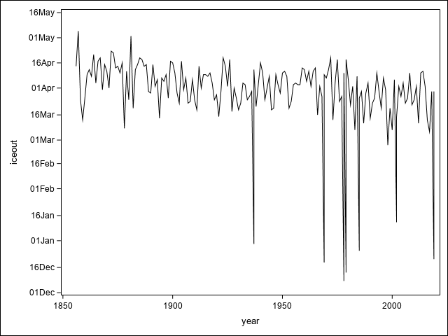

The SGPlot Procedure

There are seven suspiciously early ice out dates, which should make us look more closely at the data.

   Obs  Winter   Days  year       close        open  icein  dur  iceout

    85  1936-37     .  1937  12/07/1936  12/30/1936  07DEC   23  30DEC 
    86  1936-37   121  1937  01/05/1937  04/13/1937  05JAN   98  12APR

In some winters the lake freezes over, opens a little, then refreezes. Let's agree that we are interested in the ultimate ice out date, so we want to drop a few observations in our analysis.

Means

A simple answer to our question can be found with PROC MEANS.

proc means data=MendotaIce; * simple descriptives;
  where iceout gt "12Jan60"d;
    var iceout;
    run;

                            The MEANS Procedure

                        Analysis Variable : iceout 
 
      N            Mean         Std Dev         Minimum         Maximum
    -------------------------------------------------------------------
    164      92.3414634      11.6768551      57.0000000     125.0000000
    -------------------------------------------------------------------

Over the last 150+ years, the ice usually breaks up around the 92nd or 93rd day of the year.

We could apply our date format to interpret these results more easily.

                                  iceout

                                  02APR

The hefty standard deviation tells us we have to allow a large margin of error in guessing an ice out date.

To see the distribution of the ice out date, we can use a PROC step that produces graphs.

proc sgplot data=MendotaIce;
  where iceout gt "12Jan60"d;
    histogram iceout;
  density iceout /type=kernel;
    run;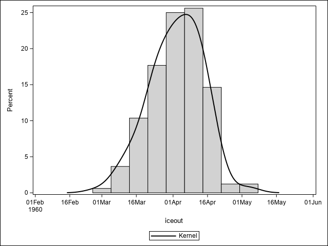

The SGPlot Procedure

Freq

Many procedures produce both tables and plots. To look at the distribution of ice out by month we could do this:

proc freq data=MendotaIce;
  where iceout gt "12Jan60"d;
    tables iceout / plots=freqplot;
    format iceout monname.;
    run;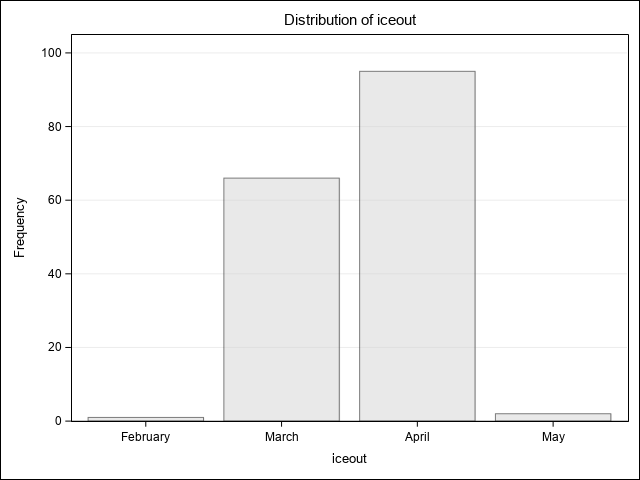

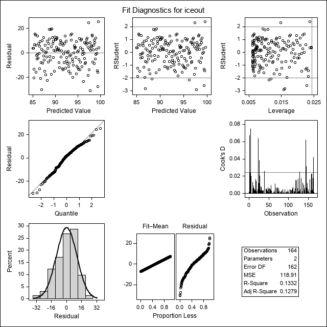
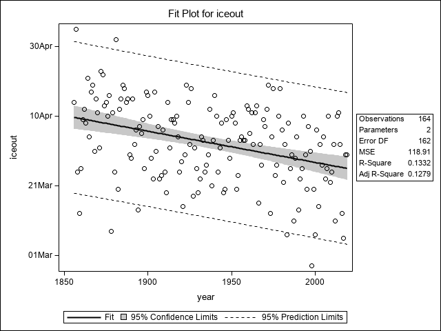
iceout	Frequency	Percent	Cumulative Frequency	Cumulative Percent
February	1	0.61	1	0.61
March	66	40.24	67	40.85
April	95	57.93	162	98.78
May	2	1.22	164	100.00

Bar Chart of Frequencies for iceout

Reg

Can we do better if we take global warming into account?

proc reg data=MendotaIce;
  where iceout gt "12Jan60"d;
    model iceout = year;
    run; quit;

Model: MODEL1

Dependent Variable: iceout

Number of Observations Read	164
Number of Observations Used	164

Analysis of Variance
Source	DF	Sum of Squares	Mean Square	F Value	Pr > F
Model	1	2961.12546	2961.12546	24.90	<.0001
Error	162	19264	118.91205
Corrected Total	163	22225

Root MSE	10.90468	R-Square	0.1332
Dependent Mean	92.34146	Adj R-Sq	0.1279
Coeff Var	11.80908

Parameter Estimates
Variable	DF	Parameter Estimate	Standard Error	t Value	Pr > \|t\|
Intercept	1	266.24285	34.85918	7.64	<.0001
year	1	-0.08976	0.01799	-4.99	<.0001

Model: MODEL1

Dependent Variable: iceout

Panel of fit diagnostics for iceout.

Scatter plot of residuals by year for iceout.

Scatterplot of iceout by year overlaid with the fit line, a 95% confidence band and lower and upper 95% prediction limits.

What does the intercept, about 270, mean?

                                 Estimate

                                  23SEP

While mathematically correct, and usable to calculate a prediction for 2020, it might make sense to rescale year to simply give us our answer.

data recentered;
    set mendotaice;
    yearc = year-2020;
    run;

Notice that the intercept changes but the slope does not.

proc reg data=recentered plots=none;
  where iceout gt "12Jan60"d;
    model iceout = yearc;
    run; quit;

Model: MODEL1

Dependent Variable: iceout

Number of Observations Read	164
Number of Observations Used	164

Analysis of Variance
Source	DF	Sum of Squares	Mean Square	F Value	Pr > F
Model	1	2961.12546	2961.12546	24.90	<.0001
Error	162	19264	118.91205
Corrected Total	163	22225

Root MSE	10.90468	R-Square	0.1332
Dependent Mean	92.34146	Adj R-Sq	0.1279
Coeff Var	11.80908

Parameter Estimates
Variable	DF	Parameter Estimate	Standard Error	t Value	Pr > \|t\|
Intercept	1	84.93663	1.71084	49.65	<.0001
yearc	1	-0.08976	0.01799	-4.99	<.0001

Now the intercept means the expected ice out date for this year:

                                 Estimate

                                  25MAR

About a week earlier than if we ignore the trend.

Over the course of a lifetime, ice fishing season had ended about a week earlier, and winter is about two weeks shorter.