First, load some example data and look at it.
load(url("http://www.ssc.wisc.edu/~hemken/Rworkshops/hsb.RData"))

head(hsb)
## id gender race ses schtyp prog read write math science socst
## 1 70 male white low public general 57 52 41 47 57
## 2 121 female white middle public vocation 68 59 53 63 61
## 3 86 male white high public general 44 33 54 58 31
## 4 141 male white high public vocation 63 44 47 53 56
## 5 172 male white middle public academic 47 52 57 53 61
## 6 113 male white middle public academic 44 52 51 63 61Many commands in R are specified in terms of formulas. A formula has a tilde ( ~ ), and terms on the left-hand side or right-hand side are composed of object names (usually existing vectors/ variables/columns in a data frame, but this can also include matrices, or the results of embedded functions like log()). Terms are connected by a variety of math-like symbols that have their own algebra.
Formulas have their own distinct class, and can even be saved as formula objects.
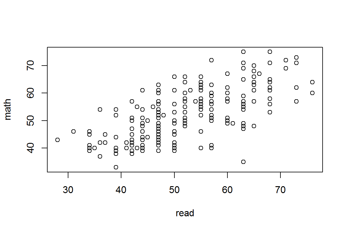
For example, a scatterplot can be specified as a formula within the plot() function. Where we can specify the relations between variables using a formula, we can almost always also specify a data= parameter to point to the source of the variables.
plot(math ~ read, data=hsb)
class(math ~ read)## [1] "formula"Formulas are the central element in specifying regression models, using lm() and a variety of other modeling functions.
# add a regression line to the plot
plot(math ~ read, data=hsb)
abline(21.0382, 0.6051)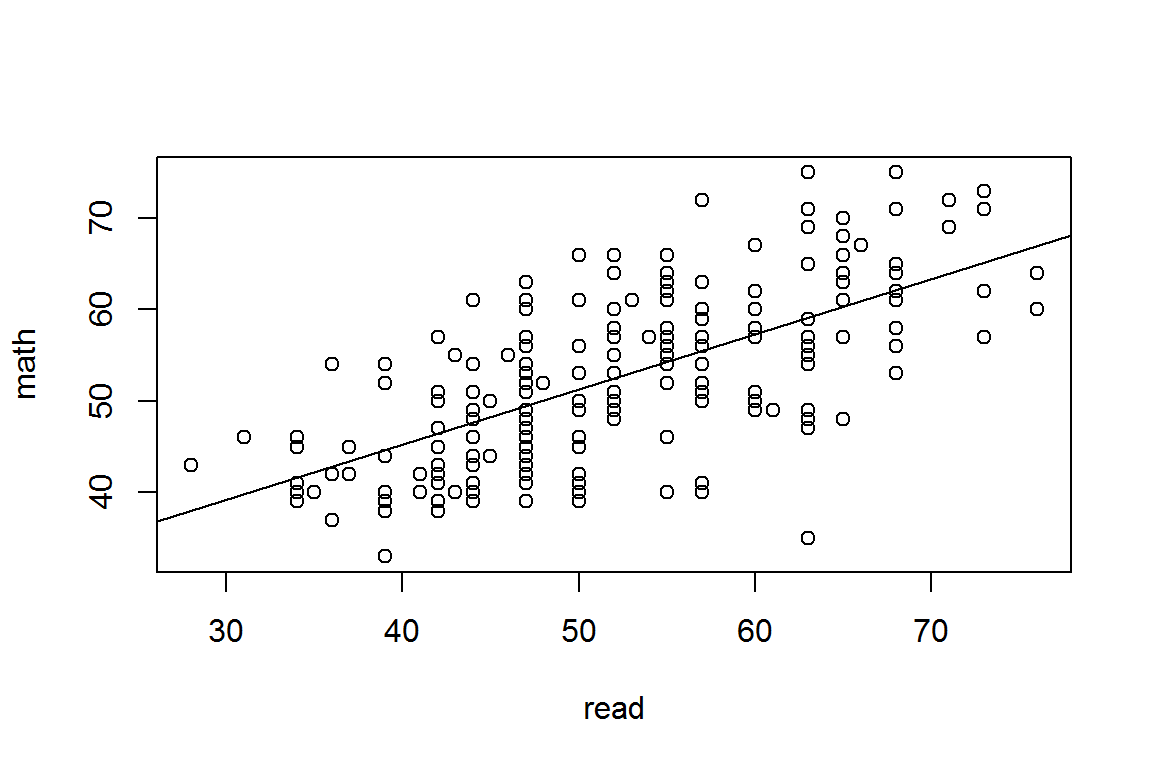
lm(math ~ read, data=hsb)##
## Call:
## lm(formula = math ~ read, data = hsb)
##
## Coefficients:
## (Intercept) read
## 21.0382 0.6051Anova models work in the same way. Note that prog is stored as a factor - this is crucial to getting the correct model.
plot(math ~ prog, data=hsb)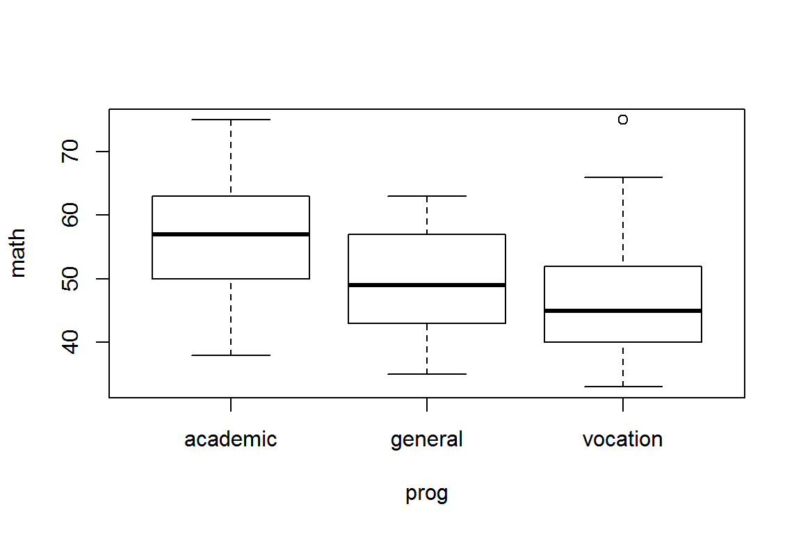
lm(math ~ prog, data=hsb)##
## Call:
## lm(formula = math ~ prog, data = hsb)
##
## Coefficients:
## (Intercept) proggeneral progvocation
## 56.733 -6.711 -10.313Notice, too, that the jargon can get confusing here. The formula is written with one term on the right-hand side, and a second term, the intercept, is assumed/implied. However, the model has three terms, the intercept and two additional levels of prog.
Sometimes we want to rearrange the levels in a factor. If we just want a different reference category, we can use relevel(). If we want to reorder all the levels, we factor() it again.
str(hsb$ses)## Factor w/ 3 levels "high","low","middle": 2 3 1 1 3 3 3 3 3 3 ...head(hsb$ses)## [1] low middle high high middle middle
## Levels: high low middlelm(math ~ ses, data=hsb)##
## Call:
## lm(formula = math ~ ses, data = hsb)
##
## Coefficients:
## (Intercept) seslow sesmiddle
## 56.172 -7.002 -3.962hsb$ses <- relevel(hsb$ses, ref="low")
lm(math ~ ses, data=hsb)##
## Call:
## lm(formula = math ~ ses, data = hsb)
##
## Coefficients:
## (Intercept) seshigh sesmiddle
## 49.170 7.002 3.040hsb$ses <- factor(hsb$ses, levels=c("low", "middle", "high"))
lm(math ~ ses, data=hsb)##
## Call:
## lm(formula = math ~ ses, data = hsb)
##
## Coefficients:
## (Intercept) sesmiddle seshigh
## 49.170 3.040 7.002A model with more than one term in the formula:
plot(math ~ read, data=hsb)
abline(27.9952, 0.5117)
abline(27.9952-3.4330, 0.5117)
abline(27.9952-5.2158, 0.5117)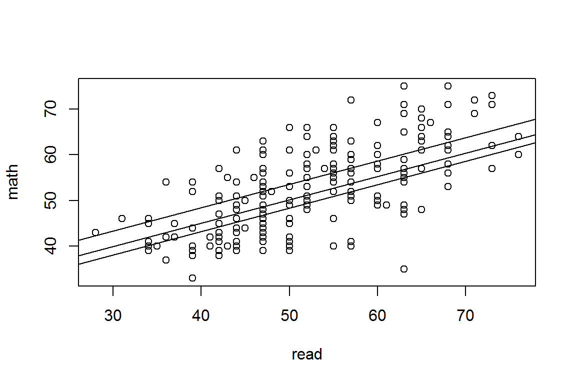
lm(math ~ prog + read, data=hsb)##
## Call:
## lm(formula = math ~ prog + read, data = hsb)
##
## Coefficients:
## (Intercept) proggeneral progvocation read
## 27.9952 -3.4330 -5.2158 0.5117Interactions may be specified a couple of different ways. An asterisk, *, means to include the higher order term plus all the related lower order terms. Alternatively, specific interaction terms may be specified with the colon, :.
plot(math ~ read, data=hsb)
abline(21.3612, 0.6298)
abline(21.3612+12.8386, 0.6298-0.3118)
abline(21.3612+6.2033, 0.6298-0.2217)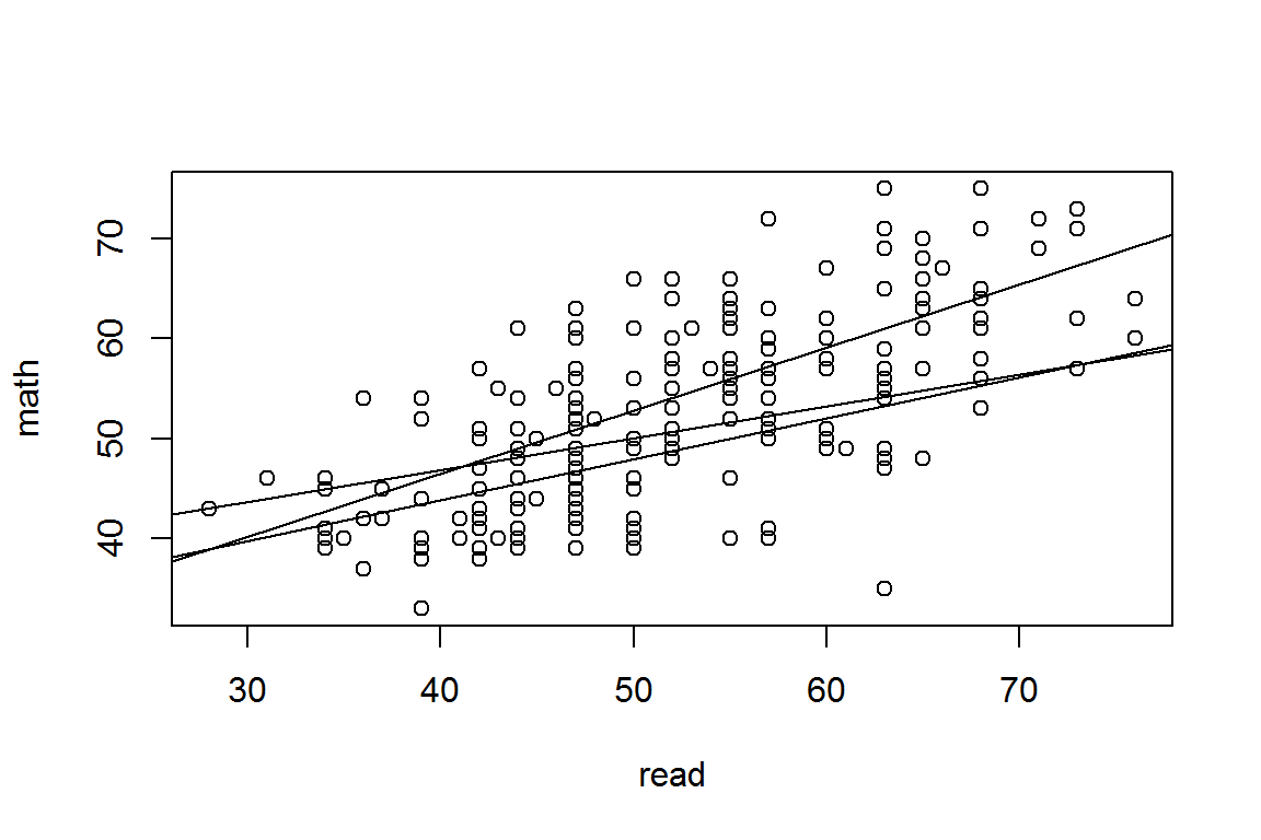
lm(math ~ prog * read, data=hsb)##
## Call:
## lm(formula = math ~ prog * read, data = hsb)
##
## Coefficients:
## (Intercept) proggeneral progvocation
## 21.3612 12.8386 6.2033
## read proggeneral:read progvocation:read
## 0.6298 -0.3118 -0.2217# the same model
lm(math ~ prog + read + prog:read, data=hsb)##
## Call:
## lm(formula = math ~ prog + read + prog:read, data = hsb)
##
## Coefficients:
## (Intercept) proggeneral progvocation
## 21.3612 12.8386 6.2033
## read proggeneral:read progvocation:read
## 0.6298 -0.3118 -0.2217Models may be modified - terms added or removed - through the use of the update() function. In this context, a period, ., represents all the terms included in the previous model.
m1 <- lm(math ~ prog * read, data=hsb)
summary(m1)
##
## Call:
## lm(formula = math ~ prog * read, data = hsb)
##
## Residuals:
## Min 1Q Median 3Q Max
## -19.2340 -5.1950 -0.1676 4.8836 21.7235
##
## Coefficients:
## Estimate Std. Error t value Pr(>|t|)
## (Intercept) 21.36122 3.88854 5.493 1.23e-07 ***
## proggeneral 12.83861 6.74579 1.903 0.0585 .
## progvocation 6.20329 6.36169 0.975 0.3307
## read 0.62982 0.06826 9.227 < 2e-16 ***
## proggeneral:read -0.31182 0.12858 -2.425 0.0162 *
## progvocation:read -0.22170 0.12696 -1.746 0.0824 .
## ---
## Signif. codes: 0 '***' 0.001 '**' 0.01 '*' 0.05 '.' 0.1 ' ' 1
##
## Residual standard error: 6.675 on 194 degrees of freedom
## Multiple R-squared: 0.5051, Adjusted R-squared: 0.4924
## F-statistic: 39.6 on 5 and 194 DF, p-value: < 2.2e-16m2 <- update(m1, .~.-prog:read) # removes two model terms
summary(m2)##
## Call:
## lm(formula = math ~ prog + read, data = hsb)
##
## Residuals:
## Min 1Q Median 3Q Max
## -21.7994 -4.6484 -0.8686 4.8846 19.9834
##
## Coefficients:
## Estimate Std. Error t value Pr(>|t|)
## (Intercept) 27.99519 2.96929 9.428 < 2e-16 ***
## proggeneral -3.43297 1.24908 -2.748 0.00655 **
## progvocation -5.21581 1.27015 -4.106 5.9e-05 ***
## read 0.51170 0.05155 9.927 < 2e-16 ***
## ---
## Signif. codes: 0 '***' 0.001 '**' 0.01 '*' 0.05 '.' 0.1 ' ' 1
##
## Residual standard error: 6.761 on 196 degrees of freedom
## Multiple R-squared: 0.487, Adjusted R-squared: 0.4792
## F-statistic: 62.03 on 3 and 196 DF, p-value: < 2.2e-16In a formula, a minus sign, -, is used to remove a term from a model.
The anova() function gives us a way to make tables of F tests. Given a single model, it returns an anova decomposition of our model. Given two or more models, it compares the models. But one caveat is that it is up to the user (you) to be sure that the models can be compared meaningfully.
anova(m1)## Analysis of Variance Table
##
## Response: math
## Df Sum Sq Mean Sq F value Pr(>F)
## prog 2 4002.1 2001.1 44.9129 < 2e-16 ***
## read 1 4504.3 4504.3 101.0973 < 2e-16 ***
## prog:read 2 315.9 158.0 3.5453 0.03074 *
## Residuals 194 8643.5 44.6
## ---
## Signif. codes: 0 '***' 0.001 '**' 0.01 '*' 0.05 '.' 0.1 ' ' 1anova(m2,m1)## Analysis of Variance Table
##
## Model 1: math ~ prog + read
## Model 2: math ~ prog * read
## Res.Df RSS Df Sum of Sq F Pr(>F)
## 1 196 8959.4
## 2 194 8643.5 2 315.91 3.5453 0.03074 *
## ---
## Signif. codes: 0 '***' 0.001 '**' 0.01 '*' 0.05 '.' 0.1 ' ' 1Another point to bear in mind is that the sums of squares reported (and therefore the F tests based on them) are the "type 1" (sequential or experimentalist's) sums of squares. For the "type 2" or "type 3" sums of squares more commonly used in the analysis of observational data, use the Anova() function (capitalized) from the car package (Companion to Applied Regression).
library(car)
Anova(m1)
## Anova Table (Type II tests)
##
## Response: math
## Sum Sq Df F value Pr(>F)
## prog 845.6 2 9.4900 0.0001169 ***
## read 4504.3 1 101.0973 < 2.2e-16 ***
## prog:read 315.9 2 3.5453 0.0307446 *
## Residuals 8643.5 194
## ---
## Signif. codes: 0 '***' 0.001 '**' 0.01 '*' 0.05 '.' 0.1 ' ' 1Anova(m1, type=3)## Anova Table (Type III tests)
##
## Response: math
## Sum Sq Df F value Pr(>F)
## (Intercept) 1344.5 1 30.1772 1.228e-07 ***
## prog 166.1 2 1.8640 0.15781
## read 3793.1 1 85.1356 < 2.2e-16 ***
## prog:read 315.9 2 3.5453 0.03074 *
## Residuals 8643.5 194
## ---
## Signif. codes: 0 '***' 0.001 '**' 0.01 '*' 0.05 '.' 0.1 ' ' 1In formulas, the plus sign, +, means to add terms, but we may also want to represent simple elementwise addition of vectors in a formula. For example, one way to constrain the coefficients of several model terms to be equal is to combine the variables into a single model term. To do this, we use the inhibit function, I(). Expressions within the I() function are interpreted as general R expressions, and not as terms within the formula.
m3 <- lm(math ~ read+write+science+socst, hsb)
coefficients(m3) # to see why we might think they are equal
## (Intercept) read write science socst
## 8.96274058 0.27068453 0.22616140 0.25389639 0.08480508m4 <- lm(math ~ I(read+write+science)+socst, hsb)
anova(m4, m3)## Analysis of Variance Table
##
## Model 1: math ~ I(read + write + science) + socst
## Model 2: math ~ read + write + science + socst
## Res.Df RSS Df Sum of Sq F Pr(>F)
## 1 197 7699.2
## 2 195 7691.3 2 7.9174 0.1004 0.9046The expression within I() becomes a single formula term, which may expand into multiple model terms.
m5 <- lm(math ~ I(read+write+science)*socst, hsb)
summary(m5)
##
## Call:
## lm(formula = math ~ I(read + write + science) * socst, data = hsb)
##
## Residuals:
## Min 1Q Median 3Q Max
## -20.5873 -4.0466 -0.1618 4.3809 15.1761
##
## Coefficients:
## Estimate Std. Error t value Pr(>|t|)
## (Intercept) 34.960338 12.925968 2.705 0.00744 **
## I(read + write + science) 0.079293 0.086220 0.920 0.35888
## socst -0.430386 0.254115 -1.694 0.09192 .
## I(read + write + science):socst 0.003310 0.001598 2.072 0.03962 *
## ---
## Signif. codes: 0 '***' 0.001 '**' 0.01 '*' 0.05 '.' 0.1 ' ' 1
##
## Residual standard error: 6.2 on 196 degrees of freedom
## Multiple R-squared: 0.5686, Adjusted R-squared: 0.562
## F-statistic: 86.12 on 3 and 196 DF, p-value: < 2.2e-16Polynomials
lm(math ~ read + read:read, data=hsb)##
## Call:
## lm(formula = math ~ read + read:read, data = hsb)
##
## Coefficients:
## (Intercept) read
## 21.0382 0.6051lm(math ~ read + I(read*read), data=hsb)##
## Call:
## lm(formula = math ~ read + I(read * read), data = hsb)
##
## Coefficients:
## (Intercept) read I(read * read)
## 24.056044 0.487359 0.001106m6 <- lm(math ~ read + I(read^2), data=hsb)
summary(m6)##
## Call:
## lm(formula = math ~ read + I(read^2), data = hsb)
##
## Residuals:
## Min 1Q Median 3Q Max
## -24.1513 -5.1513 -0.3595 4.7302 16.5695
##
## Coefficients:
## Estimate Std. Error t value Pr(>|t|)
## (Intercept) 24.056044 11.592589 2.075 0.0393 *
## read 0.487359 0.443661 1.098 0.2733
## I(read^2) 0.001106 0.004142 0.267 0.7897
## ---
## Signif. codes: 0 '***' 0.001 '**' 0.01 '*' 0.05 '.' 0.1 ' ' 1
##
## Residual standard error: 7.054 on 197 degrees of freedom
## Multiple R-squared: 0.4388, Adjusted R-squared: 0.4331
## F-statistic: 77.02 on 2 and 197 DF, p-value: < 2.2e-16Orthogonal polynomials, easier to estimate, harder to interpret.
m7 <- lm(math ~ poly(read, 2), data=hsb)
summary(m7)
##
## Call:
## lm(formula = math ~ poly(read, 2), data = hsb)
##
## Residuals:
## Min 1Q Median 3Q Max
## -24.1513 -5.1513 -0.3595 4.7302 16.5695
##
## Coefficients:
## Estimate Std. Error t value Pr(>|t|)
## (Intercept) 52.6450 0.4988 105.550 <2e-16 ***
## poly(read, 2)1 87.5258 7.0536 12.409 <2e-16 ***
## poly(read, 2)2 1.8841 7.0536 0.267 0.79
## ---
## Signif. codes: 0 '***' 0.001 '**' 0.01 '*' 0.05 '.' 0.1 ' ' 1
##
## Residual standard error: 7.054 on 197 degrees of freedom
## Multiple R-squared: 0.4388, Adjusted R-squared: 0.4331
## F-statistic: 77.02 on 2 and 197 DF, p-value: < 2.2e-16anova(m6, m7)## Analysis of Variance Table
##
## Model 1: math ~ read + I(read^2)
## Model 2: math ~ poly(read, 2)
## Res.Df RSS Df Sum of Sq F Pr(>F)
## 1 197 9801.5
## 2 197 9801.5 0 -1.6371e-11Centered data: easier to interpret, somewhat easier to estimate.
readc <- hsb$read - mean(hsb$read)
m8 <- lm(math ~ readc + I(readc^2), data=hsb)
summary(m8)
##
## Call:
## lm(formula = math ~ readc + I(readc^2), data = hsb)
##
## Residuals:
## Min 1Q Median 3Q Max
## -24.1513 -5.1513 -0.3595 4.7302 16.5695
##
## Coefficients:
## Estimate Std. Error t value Pr(>|t|)
## (Intercept) 52.529265 0.660686 79.507 <2e-16 ***
## readc 0.602942 0.049462 12.190 <2e-16 ***
## I(readc^2) 0.001106 0.004142 0.267 0.79
## ---
## Signif. codes: 0 '***' 0.001 '**' 0.01 '*' 0.05 '.' 0.1 ' ' 1
##
## Residual standard error: 7.054 on 197 degrees of freedom
## Multiple R-squared: 0.4388, Adjusted R-squared: 0.4331
## F-statistic: 77.02 on 2 and 197 DF, p-value: < 2.2e-16anova(m6,m7,m8)## Analysis of Variance Table
##
## Model 1: math ~ read + I(read^2)
## Model 2: math ~ poly(read, 2)
## Model 3: math ~ readc + I(readc^2)
## Res.Df RSS Df Sum of Sq F Pr(>F)
## 1 197 9801.5
## 2 197 9801.5 0 -1.6371e-11
## 3 197 9801.5 0 0.0000e+00Limiting higher order interactions
m9 <- lm(math ~ read*write*science*socst, data=hsb)
summary(m9)
##
## Call:
## lm(formula = math ~ read * write * science * socst, data = hsb)
##
## Residuals:
## Min 1Q Median 3Q Max
## -16.4737 -4.2876 0.1648 4.0328 14.4510
##
## Coefficients:
## Estimate Std. Error t value Pr(>|t|)
## (Intercept) 2.078e+02 3.182e+02 0.653 0.515
## read -4.123e+00 6.771e+00 -0.609 0.543
## write -7.674e+00 7.286e+00 -1.053 0.294
## science -3.305e-01 6.410e+00 -0.052 0.959
## socst -6.199e-01 6.558e+00 -0.095 0.925
## read:write 1.655e-01 1.496e-01 1.107 0.270
## read:science 2.055e-02 1.350e-01 0.152 0.879
## write:science 9.100e-02 1.410e-01 0.645 0.519
## read:socst 3.408e-02 1.367e-01 0.249 0.803
## write:socst 8.463e-02 1.379e-01 0.614 0.540
## science:socst -4.744e-02 1.291e-01 -0.367 0.714
## read:write:science -1.976e-03 2.877e-03 -0.687 0.493
## read:write:socst -2.045e-03 2.762e-03 -0.740 0.460
## read:science:socst 5.008e-04 2.634e-03 0.190 0.849
## write:science:socst -5.019e-04 2.630e-03 -0.191 0.849
## read:write:science:socst 1.785e-05 5.207e-05 0.343 0.732
##
## Residual standard error: 6.227 on 184 degrees of freedom
## Multiple R-squared: 0.5915, Adjusted R-squared: 0.5582
## F-statistic: 17.76 on 15 and 184 DF, p-value: < 2.2e-16m10 <- lm(math ~ (read+write+science+socst)^3, data=hsb)
summary(m10)##
## Call:
## lm(formula = math ~ (read + write + science + socst)^3, data = hsb)
##
## Residuals:
## Min 1Q Median 3Q Max
## -16.3854 -4.1843 0.0599 4.0885 14.4857
##
## Coefficients:
## Estimate Std. Error t value Pr(>|t|)
## (Intercept) 1.022e+02 7.919e+01 1.290 0.1986
## read -1.906e+00 1.994e+00 -0.955 0.3406
## write -5.356e+00 2.703e+00 -1.982 0.0490 *
## science 1.779e+00 1.789e+00 0.995 0.3212
## socst 1.488e+00 2.269e+00 0.656 0.5126
## read:write 1.176e-01 5.313e-02 2.214 0.0281 *
## read:science -2.365e-02 3.982e-02 -0.594 0.5532
## read:socst -9.768e-03 4.806e-02 -0.203 0.8392
## write:science 4.569e-02 4.883e-02 0.936 0.3507
## write:socst 3.964e-02 4.218e-02 0.940 0.3486
## science:socst -8.926e-02 4.223e-02 -2.114 0.0359 *
## read:write:science -1.042e-03 9.172e-04 -1.136 0.2574
## read:write:socst -1.124e-03 6.389e-04 -1.759 0.0802 .
## read:science:socst 1.368e-03 7.314e-04 1.870 0.0631 .
## write:science:socst 3.725e-04 6.368e-04 0.585 0.5593
## ---
## Signif. codes: 0 '***' 0.001 '**' 0.01 '*' 0.05 '.' 0.1 ' ' 1
##
## Residual standard error: 6.212 on 185 degrees of freedom
## Multiple R-squared: 0.5912, Adjusted R-squared: 0.5603
## F-statistic: 19.11 on 14 and 185 DF, p-value: < 2.2e-16m11 <- lm(math ~ (read+write+science+socst)^2, data=hsb)
anova(m10,m11)## Analysis of Variance Table
##
## Model 1: math ~ (read + write + science + socst)^3
## Model 2: math ~ (read + write + science + socst)^2
## Res.Df RSS Df Sum of Sq F Pr(>F)
## 1 185 7139.2
## 2 189 7375.3 -4 -236.09 1.5295 0.1954summary(m11)##
## Call:
## lm(formula = math ~ (read + write + science + socst)^2, data = hsb)
##
## Residuals:
## Min 1Q Median 3Q Max
## -19.4705 -4.2089 -0.0629 4.1309 15.1892
##
## Coefficients:
## Estimate Std. Error t value Pr(>|t|)
## (Intercept) 45.9772403 16.0937548 2.857 0.00476 **
## read -0.0041504 0.4262509 -0.010 0.99224
## write -0.6728462 0.4614207 -1.458 0.14644
## science 0.0893936 0.3644276 0.245 0.80649
## socst -0.0434814 0.3869145 -0.112 0.91064
## read:write 0.0063856 0.0090835 0.703 0.48293
## read:science -0.0054363 0.0071827 -0.757 0.45008
## read:socst 0.0038652 0.0068955 0.561 0.57578
## write:science 0.0107600 0.0082152 1.310 0.19187
## write:socst 0.0008474 0.0069352 0.122 0.90288
## science:socst -0.0022118 0.0078241 -0.283 0.77772
## ---
## Signif. codes: 0 '***' 0.001 '**' 0.01 '*' 0.05 '.' 0.1 ' ' 1
##
## Residual standard error: 6.247 on 189 degrees of freedom
## Multiple R-squared: 0.5777, Adjusted R-squared: 0.5554
## F-statistic: 25.86 on 10 and 189 DF, p-value: < 2.2e-16anova(m3,m11)## Analysis of Variance Table
##
## Model 1: math ~ read + write + science + socst
## Model 2: math ~ (read + write + science + socst)^2
## Res.Df RSS Df Sum of Sq F Pr(>F)
## 1 195 7691.3
## 2 189 7375.3 6 315.98 1.3496 0.2372The use of the poly() function brings up another side-light. Matrices may be used a formula terms, where each matrix column becomes a model term.
m <- matrix(runif(200), ncol=5)
lm(m[,1] ~ m[,2:5])
##
## Call:
## lm(formula = m[, 1] ~ m[, 2:5])
##
## Coefficients:
## (Intercept) m[, 2:5]1 m[, 2:5]2 m[, 2:5]3 m[, 2:5]4
## 0.25144 0.27210 0.05635 0.16750 -0.06199Step by step checks for a group of variables
add1(m3, scope = ~ .+gender+race+ses+schtyp+prog, data=hsb, test="F")## Single term additions
##
## Model:
## math ~ read + write + science + socst
## Df Sum of Sq RSS AIC F value Pr(>F)
## <none> 7691.3 739.91
## gender 1 40.22 7651.1 740.86 1.0199 0.3138022
## race 3 182.35 7509.0 741.11 1.5542 0.2019249
## ses 2 18.26 7673.1 743.43 0.2296 0.7950576
## schtyp 1 5.08 7686.2 741.77 0.1282 0.7206863
## prog 2 551.44 7139.9 729.03 7.4531 0.0007622 ***
## ---
## Signif. codes: 0 '***' 0.001 '**' 0.01 '*' 0.05 '.' 0.1 ' ' 1m12 <- lm(math ~ ., hsb)
anova(m12)## Analysis of Variance Table
##
## Response: math
## Df Sum Sq Mean Sq F value Pr(>F)
## id 1 839.5 839.5 22.6753 3.861e-06 ***
## gender 1 1.8 1.8 0.0496 0.8239642
## race 3 1098.6 366.2 9.8913 4.418e-06 ***
## ses 2 740.6 370.3 10.0018 7.507e-05 ***
## schtyp 1 6.8 6.8 0.1833 0.6690919
## prog 2 2934.7 1467.3 39.6352 4.720e-15 ***
## read 1 3665.5 3665.5 99.0110 < 2.2e-16 ***
## write 1 760.5 760.5 20.5431 1.044e-05 ***
## science 1 544.9 544.9 14.7177 0.0001712 ***
## socst 1 24.1 24.1 0.6509 0.4208275
## Residuals 185 6848.9 37.0
## ---
## Signif. codes: 0 '***' 0.001 '**' 0.01 '*' 0.05 '.' 0.1 ' ' 1drop1(m12, test="F")## Single term deletions
##
## Model:
## math ~ id + gender + race + ses + schtyp + prog + read + write +
## science + socst
## Df Sum of Sq RSS AIC F value Pr(>F)
## <none> 6848.9 736.71
## id 1 72.31 6921.2 736.81 1.9531 0.1639240
## gender 1 11.35 6860.3 735.04 0.3067 0.5804072
## race 3 251.00 7099.9 737.90 2.2599 0.0829589 .
## ses 2 2.76 6851.7 732.79 0.0372 0.9634694
## schtyp 1 41.84 6890.8 735.92 1.1301 0.2891458
## prog 2 493.14 7342.1 746.61 6.6602 0.0016103 **
## read 1 499.61 7348.5 748.79 13.4954 0.0003130 ***
## write 1 225.92 7074.8 741.20 6.1026 0.0144042 *
## science 1 548.59 7397.5 750.12 14.8184 0.0001629 ***
## socst 1 24.10 6873.0 735.41 0.6509 0.4208275
## ---
## Signif. codes: 0 '***' 0.001 '**' 0.01 '*' 0.05 '.' 0.1 ' ' 1step(m12)## Start: AIC=736.71
## math ~ id + gender + race + ses + schtyp + prog + read + write +
## science + socst
##
## Df Sum of Sq RSS AIC
## - ses 2 2.76 6851.7 732.79
## - gender 1 11.35 6860.3 735.04
## - socst 1 24.10 6873.0 735.41
## - schtyp 1 41.84 6890.8 735.92
## <none> 6848.9 736.71
## - id 1 72.31 6921.2 736.81
## - race 3 251.00 7099.9 737.90
## - write 1 225.92 7074.8 741.20
## - prog 2 493.14 7342.1 746.61
## - read 1 499.61 7348.5 748.79
## - science 1 548.59 7397.5 750.12
##
## Step: AIC=732.79
## math ~ id + gender + race + schtyp + prog + read + write + science +
## socst
##
## Df Sum of Sq RSS AIC
## - gender 1 12.87 6864.5 731.16
## - socst 1 28.62 6880.3 731.62
## - schtyp 1 39.66 6891.3 731.94
## <none> 6851.7 732.79
## - id 1 71.99 6923.7 732.88
## - race 3 254.54 7106.2 734.08
## - write 1 223.57 7075.2 737.21
## - prog 2 501.88 7353.6 742.92
## - read 1 498.21 7349.9 744.82
## - science 1 555.39 7407.1 746.37
##
## Step: AIC=731.16
## math ~ id + race + schtyp + prog + read + write + science + socst
##
## Df Sum of Sq RSS AIC
## - socst 1 28.48 6893.0 729.99
## - schtyp 1 44.02 6908.6 730.44
## <none> 6864.5 731.16
## - id 1 82.68 6947.2 731.56
## - race 3 262.00 7126.5 732.65
## - write 1 216.83 7081.4 735.38
## - prog 2 511.73 7376.3 741.54
## - read 1 530.98 7395.5 744.06
## - science 1 625.46 7490.0 746.60
##
## Step: AIC=729.99
## math ~ id + race + schtyp + prog + read + write + science
##
## Df Sum of Sq RSS AIC
## - schtyp 1 50.96 6944.0 729.46
## <none> 6893.0 729.99
## - id 1 95.12 6988.1 730.73
## - race 3 253.37 7146.4 731.21
## - write 1 303.61 7196.6 736.61
## - prog 2 569.55 7462.6 741.87
## - science 1 625.17 7518.2 745.35
## - read 1 695.81 7588.8 747.22
##
## Step: AIC=729.46
## math ~ id + race + prog + read + write + science
##
## Df Sum of Sq RSS AIC
## - id 1 45.51 6989.5 728.77
## <none> 6944.0 729.46
## - race 3 213.13 7157.1 729.51
## - write 1 288.99 7233.0 735.62
## - prog 2 552.13 7496.1 740.76
## - read 1 656.84 7600.8 745.54
## - science 1 698.22 7642.2 746.62
##
## Step: AIC=728.77
## math ~ race + prog + read + write + science
##
## Df Sum of Sq RSS AIC
## - race 3 173.13 7162.6 727.66
## <none> 6989.5 728.77
## - write 1 290.10 7279.6 734.90
## - prog 2 637.13 7626.6 742.22
## - read 1 612.74 7602.2 743.58
## - science 1 762.98 7752.5 747.49
##
## Step: AIC=727.66
## math ~ prog + read + write + science
##
## Df Sum of Sq RSS AIC
## <none> 7162.6 727.66
## - write 1 395.93 7558.6 736.42
## - prog 2 615.92 7778.5 740.16
## - read 1 581.00 7743.6 741.26
## - science 1 845.74 8008.4 747.98##
## Call:
## lm(formula = math ~ prog + read + write + science, data = hsb)
##
## Coefficients:
## (Intercept) proggeneral progvocation read write
## 16.5056 -3.7924 -4.1233 0.2401 0.2015
## science
## 0.2863step(m12, direction="both")## Start: AIC=736.71
## math ~ id + gender + race + ses + schtyp + prog + read + write +
## science + socst
##
## Df Sum of Sq RSS AIC
## - ses 2 2.76 6851.7 732.79
## - gender 1 11.35 6860.3 735.04
## - socst 1 24.10 6873.0 735.41
## - schtyp 1 41.84 6890.8 735.92
## <none> 6848.9 736.71
## - id 1 72.31 6921.2 736.81
## - race 3 251.00 7099.9 737.90
## - write 1 225.92 7074.8 741.20
## - prog 2 493.14 7342.1 746.61
## - read 1 499.61 7348.5 748.79
## - science 1 548.59 7397.5 750.12
##
## Step: AIC=732.79
## math ~ id + gender + race + schtyp + prog + read + write + science +
## socst
##
## Df Sum of Sq RSS AIC
## - gender 1 12.87 6864.5 731.16
## - socst 1 28.62 6880.3 731.62
## - schtyp 1 39.66 6891.3 731.94
## <none> 6851.7 732.79
## - id 1 71.99 6923.7 732.88
## - race 3 254.54 7106.2 734.08
## + ses 2 2.76 6848.9 736.71
## - write 1 223.57 7075.2 737.21
## - prog 2 501.88 7353.6 742.92
## - read 1 498.21 7349.9 744.82
## - science 1 555.39 7407.1 746.37
##
## Step: AIC=731.16
## math ~ id + race + schtyp + prog + read + write + science + socst
##
## Df Sum of Sq RSS AIC
## - socst 1 28.48 6893.0 729.99
## - schtyp 1 44.02 6908.6 730.44
## <none> 6864.5 731.16
## - id 1 82.68 6947.2 731.56
## - race 3 262.00 7126.5 732.65
## + gender 1 12.87 6851.7 732.79
## + ses 2 4.28 6860.3 735.04
## - write 1 216.83 7081.4 735.38
## - prog 2 511.73 7376.3 741.54
## - read 1 530.98 7395.5 744.06
## - science 1 625.46 7490.0 746.60
##
## Step: AIC=729.99
## math ~ id + race + schtyp + prog + read + write + science
##
## Df Sum of Sq RSS AIC
## - schtyp 1 50.96 6944.0 729.46
## <none> 6893.0 729.99
## - id 1 95.12 6988.1 730.73
## + socst 1 28.48 6864.5 731.16
## - race 3 253.37 7146.4 731.21
## + gender 1 12.73 6880.3 731.62
## + ses 2 9.72 6883.3 733.71
## - write 1 303.61 7196.6 736.61
## - prog 2 569.55 7462.6 741.87
## - science 1 625.17 7518.2 745.35
## - read 1 695.81 7588.8 747.22
##
## Step: AIC=729.46
## math ~ id + race + prog + read + write + science
##
## Df Sum of Sq RSS AIC
## - id 1 45.51 6989.5 728.77
## <none> 6944.0 729.46
## - race 3 213.13 7157.1 729.51
## + schtyp 1 50.96 6893.0 729.99
## + socst 1 35.41 6908.6 730.44
## + gender 1 17.43 6926.5 730.96
## + ses 2 4.87 6939.1 733.32
## - write 1 288.99 7233.0 735.62
## - prog 2 552.13 7496.1 740.76
## - read 1 656.84 7600.8 745.54
## - science 1 698.22 7642.2 746.62
##
## Step: AIC=728.77
## math ~ race + prog + read + write + science
##
## Df Sum of Sq RSS AIC
## - race 3 173.13 7162.6 727.66
## <none> 6989.5 728.77
## + id 1 45.51 6944.0 729.46
## + socst 1 41.22 6948.3 729.59
## + gender 1 24.26 6965.2 730.07
## + schtyp 1 1.35 6988.1 730.73
## + ses 2 8.60 6980.9 732.52
## - write 1 290.10 7279.6 734.90
## - prog 2 637.13 7626.6 742.22
## - read 1 612.74 7602.2 743.58
## - science 1 762.98 7752.5 747.49
##
## Step: AIC=727.66
## math ~ prog + read + write + science
##
## Df Sum of Sq RSS AIC
## <none> 7162.6 727.66
## + race 3 173.13 6989.5 728.77
## + socst 1 22.75 7139.9 729.03
## + gender 1 22.67 7140.0 729.03
## + id 1 5.51 7157.1 729.51
## + schtyp 1 2.91 7159.7 729.58
## + ses 2 13.79 7148.8 731.28
## - write 1 395.93 7558.6 736.42
## - prog 2 615.92 7778.5 740.16
## - read 1 581.00 7743.6 741.26
## - science 1 845.74 8008.4 747.98##
## Call:
## lm(formula = math ~ prog + read + write + science, data = hsb)
##
## Coefficients:
## (Intercept) proggeneral progvocation read write
## 16.5056 -3.7924 -4.1233 0.2401 0.2015
## science
## 0.2863