5 Numeric
5.1 Creating Vectors
Where do vectors come from? Most often, the vectors you work with will be derived from data you read in from elsewhere. (We will get to the topic of importing data later.) But in a variety of situations you will need to produce vectors from scratch, and creating vectors is a good way to understand what they are and how they are processed.
In R a vector is a one-dimensional ordered array of elements of the same type, typically numeric, character, or logical.
5.1.1 c() - Combine or Concatenate
The most basic vector is perhaps one that you create by cobbling together the individual elements.
a <- c(1, 3, 5)
a
[1] 1 3 5The type or class of the vector depends upon the elements you piece together.
b <- c("a", "b", "c")
b
[1] "a" "b" "c"

d <- c(TRUE, FALSE, TRUE)
d
[1]  TRUE FALSE  TRUE

e <- c(1, TRUE, FALSE)
e
[1] 1 1 0
In the last example, the vector e, you will notice that TRUE and FALSE
were promoted (coerced) to integers. All of the elements of a vector
must be of the same type, and where inputs to the combine function are
of mixed typed, they are promoted to the highest type. Take a moment
to look up the c function in Help, and look at the hierarchy given
in the first paragraph of the Details section.
- What would be the type in this vector? Make a prediction, and then check your answer.
f <- c(1, TRUE, FALSE, "d")5.1.2 rep() - Replicate or Repeat
Sometimes we need a vector with an element or sequence repeated.
a <- rep(0.2, times=5)
a
[1] 0.2 0.2 0.2 0.2 0.2

sum(a) # sum the elements
[1] 1
If you have more than one element to repeat, there are two ways to go about it.
a <- rep(c(0,1), each=4)
b <- rep(c(0,1), times=4)

rbind(a, b) # combine rows
  [,1] [,2] [,3] [,4] [,5] [,6] [,7] [,8]
a    0    0    0    0    1    1    1    1
b    0    1    0    1    0    1    0    1
This could be the beginnings of an experimental design: two factors (variables), each with two levels, and two repetitions of each combination.
Try it out: How would you produce a design for two factors, one with two levels and the other with three levels, and just one replication of each combination?
Try it out: Can you produce a factorial design (all combinations of all levels) for three factors, each with two levels?
5.1.3 seq() - Sequence
We have already seen the colon used as a binary operator to produce
sequences of integers. A more flexible function is seq.
seq(from=0, to=1, by=0.2)
[1] 0.0 0.2 0.4 0.6 0.8 1.0

seq(from=0, to=1, by=0.3) # the steps need not end at "to"
[1] 0.0 0.3 0.6 0.9

seq(from=1, to=0.5, by=-.1) # steps can descend
[1] 1.0 0.9 0.8 0.7 0.6 0.5

seq(from=1, to=2, length.out=6) # just specify "steps + 1" for the length.out argument
[1] 1.0 1.2 1.4 1.6 1.8 2.0- Try it out: Design an experiment with two variables. The first variable has two levels, "A" and "B", the second variable has levels from 3 to 4 in 5 equal steps. The design should have all combinations of the variables, two replicates for each combination, for 2x6x2=24 runs.
5.1.4 Random Numbers
We have seen sample used to pick random numbers out of a vector
and to produce random permutations. We can also generate random
numbers from standard probability distributions (see help("Distributions").
a <- runif(100) # the uniform distribution, with min=0 and max=1
hist(a)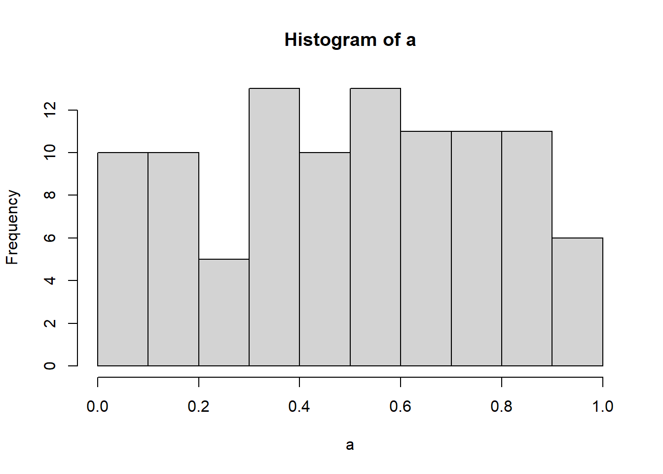
b <- rnorm(100) # the normal distribution, with mean=0 and sd=1
hist(b)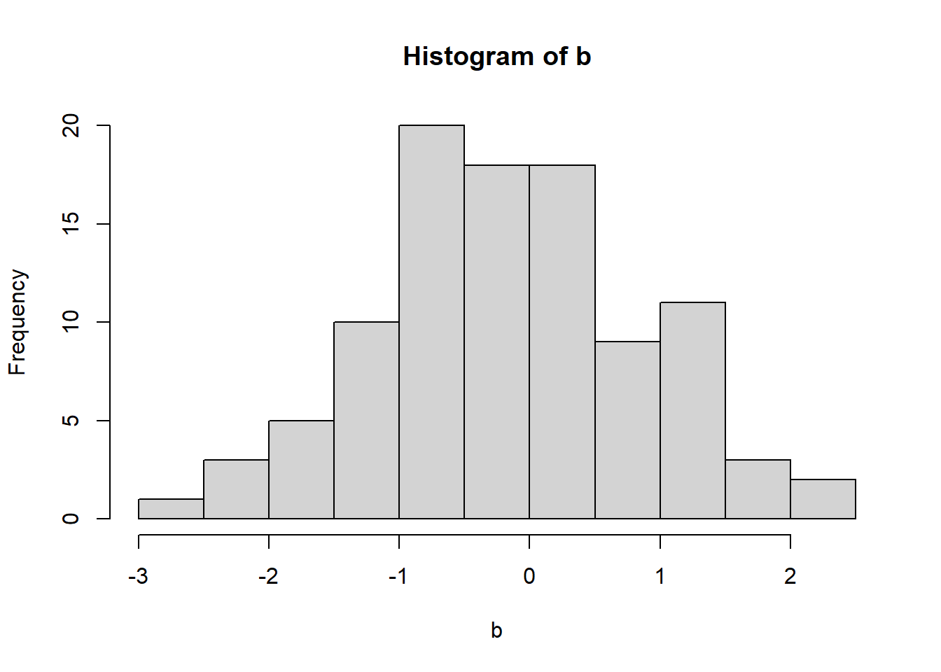
We could use some of these functions to create examples
for the t.test function.
# two sample t-test
a <- rnorm(25, mean=1, sd=1)
b <- rnorm(25, mean=3, sd=1)

t.test(a, b)
    Welch Two Sample t-test

data:  a and b
t = -4.8707, df = 45.611, p-value = 1.377e-05
alternative hypothesis: true difference in means is not equal to 0
95 percent confidence interval:
 -2.515832 -1.044244
sample estimates:
mean of x mean of y
1.148368 2.928406 - Try it out: Generate vectors from uniform distributions instead of normal distributions. Use the same means (1 and 3), but let the data range over mean-1 to mean+1.
5.2 Deleting Vectors (Cleanup)
After a while, your workspace (a.k.a. the global environment) can get cluttered. You can create a character vector with the names of objects in your workspace
ls() # alias objects() [1] "a" "b" "cmonth" "d" "dates" "e" "fmonth" "mod" "mpg" "ndays"
[11] "smonth" "tmonth" "x" "y" "z" and remove those you no longer need.
remove(a)                # alias rm()
remove("b")              # quotes are optional
remove(list=c("d", "e")) # remove several objects
remove(list=ls())        # remove everything
5.3 Vector Operations
When you are doing math or other data manipulations with several vectors, you will commonly have either several vectors of the same length, or a mix of vectors and scalars (a vector with length one). If you have experience working with statistical software, you will not be surprised that binary operations are carried out element by element:
a is c(0, 1, 2, 3, 4) and b is c(4, 3, 2, 1, 0). These will be “lined up” and operated on. The first element of the output will operate on the first element of a and the first element of b, the second element in the output will be calculated from the second elements of a and b, and so on. a + b will be c(0+4, 1+3, 2+2, 3+1, 4+0), or c(4, 4, 4, 4, 4).
a <- 0:4
b <- 4:0

a + b # addition
[1] 4 4 4 4 4
a ^ b # exponentiation
[1] 0 1 4 3 1

a * b # elementwise multiplication
[1] 0 3 4 3 0

t(a) %*% b # matrix multiplication
     [,1]
[1,]   10
It is quite possible to operate on vectors of different lengths, too.
d <- 1:4
e <- c(0,1)

d - e
[1] 1 1 3 3
In this case, the elements of the shorter vector are recycled (think rep())
to match the length of the longer vector. Where there is no remainder
(mod(length(longer), length(shorter)) == 0), R considers this an unremarkable
operation (no message from R). Where there is a remainder, you get a warning message, but you also
get a result.
d <- 0:4
e <- c(0,1)

d - e
Warning in d - e: longer object length is not a multiple of shorter object length
[1] 0 0 2 2 4
Operating on a vector and a scalar, then, works the way you probably expect. (Recall from Data Structures that scalars are vectors of length one.) The scalar is recycled/repeated to match the length of the vector, and the operation is then carried out element-wise.
d*2
[1] 0 2 4 6 8
5.4 Concatenating Vectors
You might guess that making one big vector out of two little vectors uses
the same combine function as before (c()).
For example, another (more typical) way to organize data for a two-sample t-test would be
# two sample t-test, again
a <- rnorm(25, mean=1, sd=1)
b <- rnorm(20, mean=3, sd=1)

y <- c(a,b)  # combine two vectors

x <- c(rep(0, length(a)), rep(1, length(b))) # where 0 and 1 may refer to experimental conditions

t.test(y ~ x, var.equal=TRUE) # classic t-test
    Two Sample t-test

data:  y by x
t = -6.1934, df = 43, p-value = 1.913e-07
alternative hypothesis: true difference in means is not equal to 0
95 percent confidence interval:
 -3.069775 -1.561679
sample estimates:
mean in group 0 mean in group 1
      0.8465335       3.1622605
5.5 Referencing Elements of a Vector
Often we want to work with just part of a vector, extracting or replacing part of it. You can generally refer to the elements of a data object by (1) position, (2) name, or (3) a logical condition. With vectors, this will be done with square brackets.
5.5.1 Position
If we want to select a random number, we can first create a vector with sample() and then choose one or more of its elements.
a <- sample(10)
a
[1] 3 6 5 7 1 10 4 8 9 2a[1] # pick the element in position 1[1] 3a[c(1,3,5)] # pick 3 elements[1] 3 5 1We can use this for replacement as well.
a[1] <- NA  # the missing value
a
[1] NA 6 5 7 1 10 4 8 9 2Notice that addressing a non-existent position is not an error, but it
resizes the vector, and it fills in skipped-over elements (a[11]) with NA.
a[12] <- 12
a
[1] NA 6 5 7 1 10 4 8 9 2 NA 125.5.2 Named Elements
a is not a named vector, but we can turn it into one.
names(a) <- paste0("v", 1:12)  # paste0() creates a character vector
a
v1 v2 v3 v4 v5 v6 v7 v8 v9 v10 v11 v12
NA 6 5 7 1 10 4 8 9 2 NA 12 a["v5"]v5
1 Be aware that names need not be unique, and that they can include non-alphanumeric characters. The following examples are not necessarily “good” names, but do note that there are no errors or warning messages. This can lead to trouble that is difficult to track down.
names(a)[5] <- "v (5)"
names(a)[2] <- "v1"
a
v1 v1 v3 v4 v (5) v6 v7 v8 v9 v10 v11 v12
NA 6 5 7 1 10 4 8 9 2 NA 12 a["v1"] # just the first "v1"v1
NA a[c("v1", "v1")] # grabs the same element twicev1 v1
NA NA 5.5.3 Condition
Finally, we can address the elements of a vector using logical conditions.
For example,
cond <- names(a) == "v1"
cond
[1] TRUE TRUE FALSE FALSE FALSE FALSE FALSE FALSE FALSE FALSE FALSE FALSEa[cond]v1 v1
NA 6 5.6 Numeric Vector Exercises
- Reproduce the following vector with
c()andrep():
- 1 2 1 2 1 2
- Reproduce the following vector with
seq()and a mathematical operator:
- 0 4 16 36 64 100
- Reproduce the following vector with
rep()andseq():
- -1 0 1 0 -1 0 1 0 -1 0 1 0 -1 0 1 0
- Make a vector with the numbers 1 to 10. Then, replace all the even numbers with your name.
- What was the class of the vector when it was numbers? What is it now?
- Create a vector of ten random numbers between 0 and 1, and randomly assign the names “Good” and “Bad” to the numbers.
- Bonus: Assign “Good” with probability 0.7 and “Bad” with probability 0.3.