4 Data Class
Some R functions require certain kinds of objects as arguments, while other functions can handle many kinds of objects. The latter are called generic functions.
4.1 Generic Functions
Generic functions use different methods according to the class of an object.
To view the class of an object, use the class() function:
class(mtcars)[1] "data.frame"mpg <- mtcars$mpg
class(mpg)[1] "numeric"mod <- lm(mpg ~ wt, data = mtcars)
class(mod)[1] "lm"Three commonly used generic functions are print, summary, and plot.
Each of these functions has many methods, so the output will vary depending on
the class of the object you use.
Try using the print, summary, and plot functions with mtcars, mpg,
and mod. What differences do you see?
If you use an object with a class that a function does not handle, R will be happy to give you an error, even though it may be a little cryptic:
t.test(mod)Warning in mean.default(x): argument is not numeric or logical: returning NAError in var(x): is.atomic(x) is not TRUEanova(mtcars)Error in UseMethod("anova"): no applicable method for 'anova' applied to an object of class "data.frame"On the other hand, you may be surprised at some of the objects that a function
does handle! For example, plot will produce a scatterplot matrix when
given a data.frame as input.
class(mtcars[,1:4])[1] "data.frame"plot(mtcars[,1:4])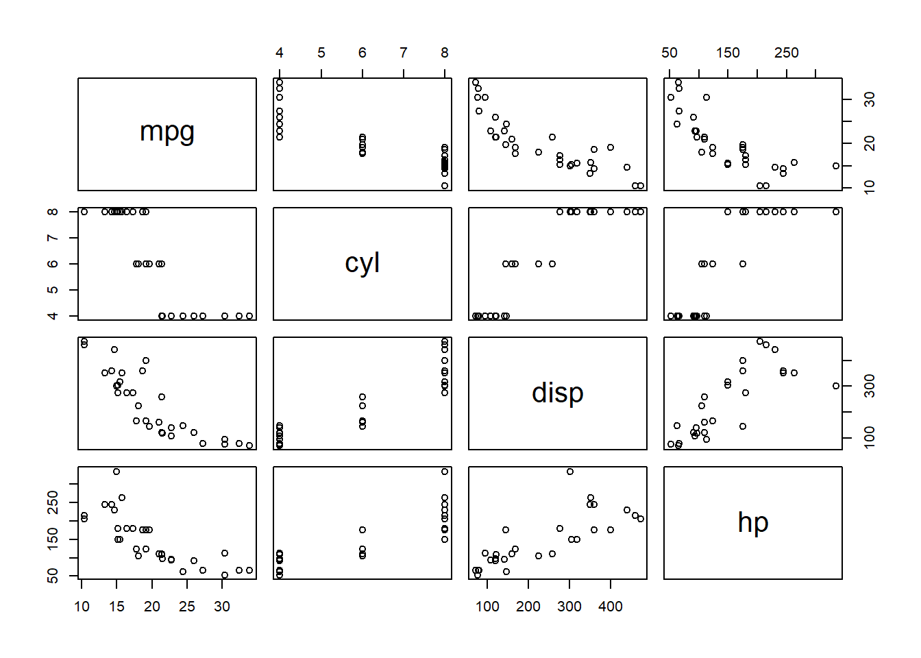
4.2 Example - Factor versus Character
Factors and dates are both numeric data, but they are processed in unique ways because of their class attributes. (These specific classes are discussed in more detail in Chapters 8 and 9.)
As an example consider a vector of 25 month names.
cmonth <- sample(month.name, 25, replace = TRUE)
fmonth <- factor(cmonth)
Here cmonth is a character vector, while fmonth
has class factor. Compare the output of the summary()
and plot() functions when applied to the character
vector versus the factor.
summary(cmonth) Length Class Mode
25 character character summary(fmonth) April August December February January July June March May
2 5 1 4 2 1 2 1 3
October September
2 2 plot(cmonth)Warning in xy.coords(x, y, xlabel, ylabel, log): NAs introduced by coercionWarning in min(x): no non-missing arguments to min; returning InfWarning in max(x): no non-missing arguments to max; returning -InfError in plot.window(...): need finite 'ylim' values
plot(fmonth)While the printed format of a data object is often a clue
as to it’s class, this is not always definitive.
In the next example, even though the output of summary(fmonth)
and table(fmonth) start with the same data and look the same,
the results are stored differently by R. The summary() function
gives us a named numeric vector, while table() gives us a table
with a numeric vector and a character vector.
tmonth <- table(fmonth)
tmonthfmonth
    April    August  December  February   January      July      June     March       May
        2         5         1         4         2         1         2         1         3
  October September
2 2 smonth <- summary(fmonth)
smonth April August December February January July June March May
2 5 1 4 2 1 2 1 3
October September
2 2 str(tmonth) 'table' int [1:11(1d)] 2 5 1 4 2 1 2 1 3 2 ...
- attr(*, "dimnames")=List of 1
..$ fmonth: chr [1:11] "April" "August" "December" "February" ...str(smonth) Named int [1:11] 2 5 1 4 2 1 2 1 3 2 ...
- attr(*, "names")= chr [1:11] "April" "August" "December" "February" ...This becomes important when used with the plot() function
which will handle these two classes in different ways.
plot(smonth)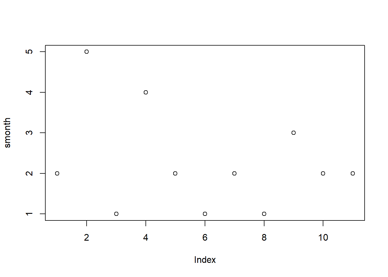
plot(tmonth)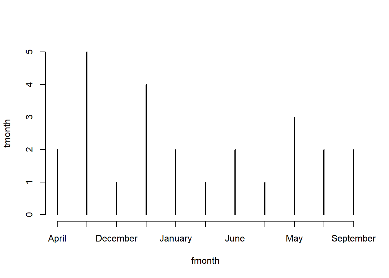
4.3 Example - Date versus Numeric
To take a closer look at dates, we can make a vector of dates
from September 1-30, 2020, with seq(). If we coerce the
date vector to numeric, we see that R stores dates as the
number of days since January 1, 1970.
dates <- seq(from = as.Date("2020-09-01"),
             to = as.Date("2020-09-30"),
             by = "days")

ndays <- as.numeric(dates)
ndays
[1] 18506 18507 18508 18509 18510 18511 18512 18513 18514 18515 18516 18517 18518 18519 18520
[16] 18521 18522 18523 18524 18525 18526 18527 18528 18529 18530 18531 18532 18533 18534 18535The generic functions we used earlier also handle dates in special ways.
Because dates are numbers, we can calculate summary statistics. There is such a thing as a “mean” date: the average of the dates’ numeric values, reconverted into a date object (and then rounded).
class(dates)[1] "Date"str(dates) Date[1:30], format: "2020-09-01" "2020-09-02" "2020-09-03" "2020-09-04" "2020-09-05" "2020-09-06" ...summary(dates) Min. 1st Qu. Median Mean 3rd Qu. Max.
"2020-09-01" "2020-09-08" "2020-09-15" "2020-09-15" "2020-09-22" "2020-09-30" summary(ndays) Min. 1st Qu. Median Mean 3rd Qu. Max.
18506 18513 18521 18521 18528 18535 plot(dates)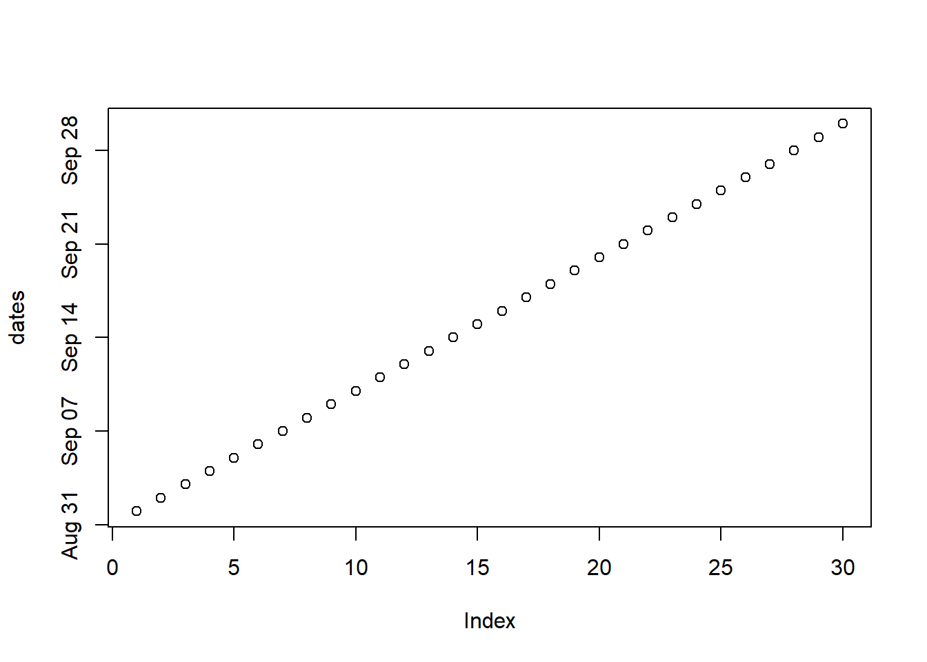
plot(ndays)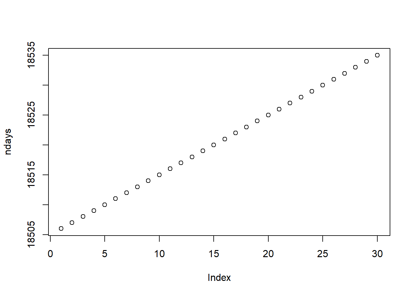
The takeaway from these illustrations is that classes play a role in how some functions handle our data, so we need to be aware of the classes of our data objects.