R Basics with RStudio
June 2021
1 Working with RStudio
R is general purpose statistical software, and like all such software, at it’s core is a programming language. The primary task with such software is to write and run code.
There are several programs you can use to edit and run R commands. The most popular of these is RStudio.
The basics elements of using an interactive interface will include:
- Writing and running commands
- Finding your results
- Saving those commands and results
Beyond these software basics, you will also need some understanding of how the programming language works. We will talk about:
- R grammar
- Using Help
- Extending R (packages)
1.1 Writing and Running Commands
There are two main panes in RStudio where we write and execute R commands, or R statements. We work with scripts – sequences of statements – in the script editor and we work with individual statements in the Console.
1.1.1 Working with Scripts
You do most of your work in RStudio by writing, running, and saving scripts, files with sequences of R statements. A good script documents your work and also makes it easy to go back and correct any mistakes you may later find.
If your project takes more than 3 to 4 statements to complete, you should probably be writing a script!
1.1.1.1 Writing Scripts
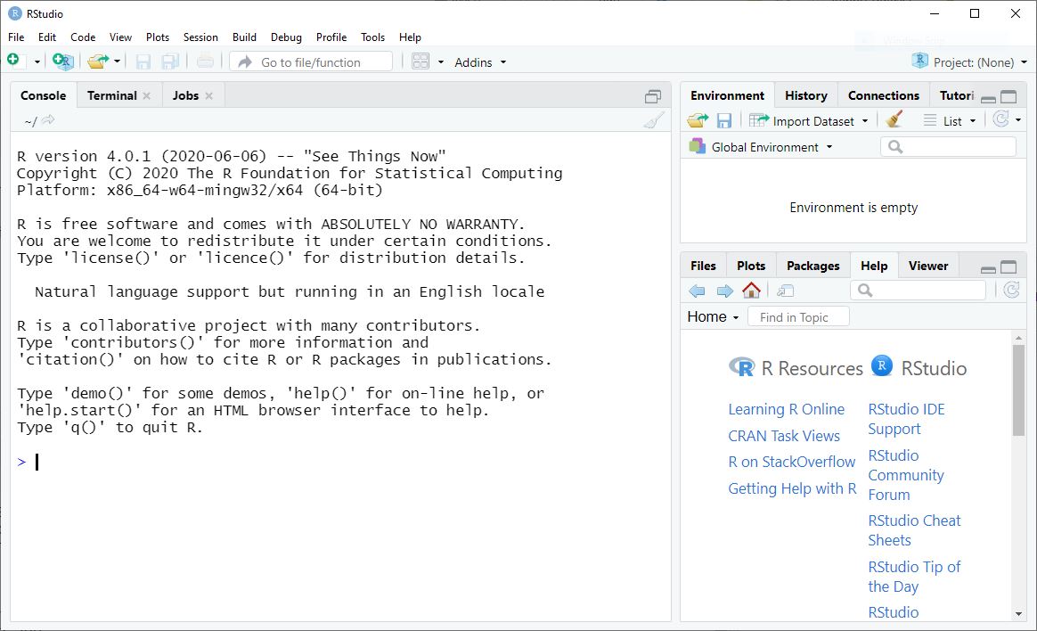
Start a new script by going to the File menu and clicking New File - R Script. You can do the same thing by clicking the New File icon on the toolbar.
You’ll notice you have the usual options for opening existing files and for saving script files in the menu and on the toolbar.
You’ll open existing scripts by clicking on them in the Files pane, in the lower right corner of the RStudio workspace.
As an example, we’ll look at a one-sample t-test. We’ll simulate the data, so we know what the result should be, then perform the test.
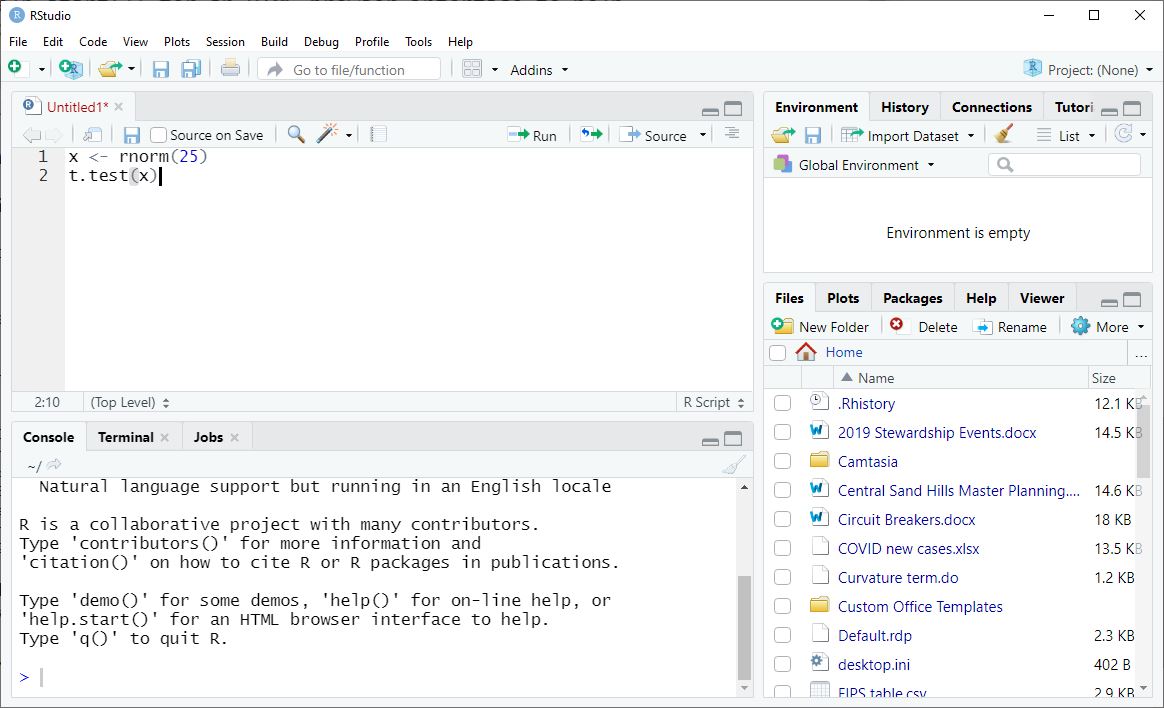
Type the following statements into a new script:
x <- rnorm(25)
t.test(x)
This generates 25 observations from a random normal distribution with mean zero and a standard deviation of one. Then we perform a one-sample t-test. We expect we won’t reject the null hypothesis that the mean is zero.
1.1.1.2 Running Scripts
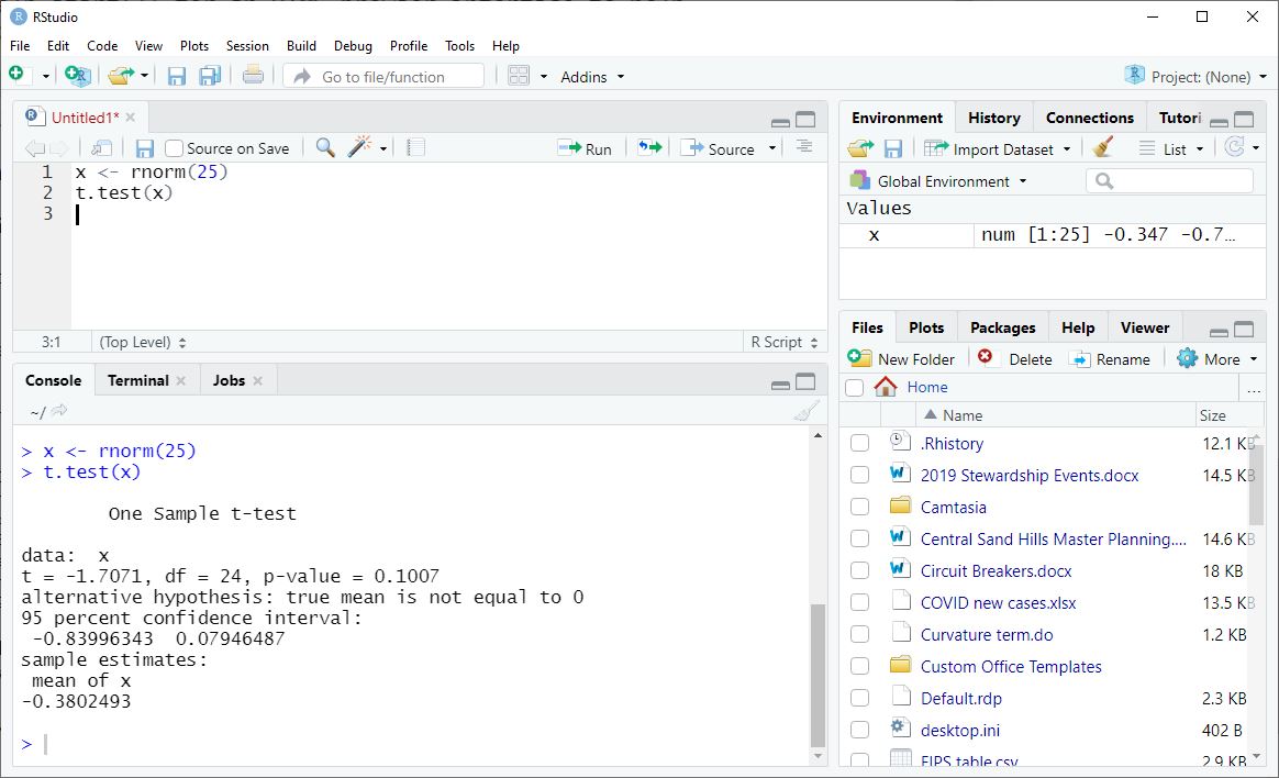
Each line in our script is a statement, a command to be run. To run these statements one at a time move your cursor anywhere in the first line and key Ctrl-Enter (or Cmd-Enter on Mac). You can also click on the Run button at the top of the script editor. Both of these actions not only run the current statement, but also move the cursor to the next statement, making it easy to walk step by step through your script.
To run more than one statement at a time, highlight all the code you want to run and then key Ctrl-Enter or click Run. (Be careful: you can highlight less than a full statement, and R will try to execute only what you highlighted!)
    One Sample t-test

data:  x
t = -2.1139, df = 24, p-value = 0.0451
alternative hypothesis: true mean is not equal to 0
95 percent confidence interval:
 -0.677665056 -0.008115103
sample estimates:
 mean of x
-0.3428901
If you try this example, you will certainly get different numbers, because we are generating random data. You might even get a result where you reject the null hypothesis! Why?
1.1.2 Working in the Console
When you are in the midst of thinking your way through a problem, you will also find it useful to issue statements in the Console. The Console is the programmer’s scratch sheet of paper.
For example, suppose you have done the first step above,
generating random numbers in a vector called x. As a
check, you decide you’d like to see the numbers generated,
and calculate their mean, which should be close to zero.
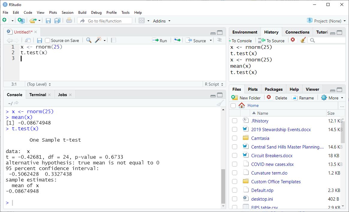
In the Console, at the > prompt, you type
x [1] -0.793791165 -1.109649993 -0.428784036 -0.080745033 -0.468762690 -0.377850538
[7] -0.558680500 -1.058771286 0.240512135 -0.677971295 0.173085540 0.185240298
[13] 0.437066956 -0.969243717 1.815949736 -1.084113230 -1.141976500 0.007661563
[19] 0.163938817 1.030609108 -0.406674653 -1.016618669 0.068388538 -2.239907602
[25] -0.281163761an implicit print() function. The numbers look reasonable
(most of the values are between -2 and 2, right?), so you
follow up in the Console with
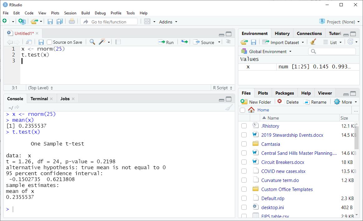
mean(x)[1] -0.3428901which is statistically close to zero. So if I now follow up
with the t.test() in my script, my result should be not
statistically significant (a p-value larger than 0.05 in the
second line of the output).
1.1.3 Command History
R keeps track of your command history, whether the statements were run from a script or from the Console. In the Console you can scroll through this history with either with the up and down arrows on your keyboard (the ones you use to move your cursor in a document).
For example, you could use feature this to quickly generate a new sample and run a new t-test by scrolling “back” (up) and executing each command in sequence.
You can also access your command history in RStudio’s History pane (upper right, tabbed with Environment). Here you can highlight one or more statements and send them to the Console. You can also send statements “to Source” (your script), turning your scratch work into something you can save.
1.1.4 Exercises - Running Commands
Try an example where you do expect to reject the null hypothesis.
Create a script where you generate random observations, and test the hypothesis that the mean is zero with a t-test.
You can generate
nrandom observations from a normal distribution with meanmand a standard deviation of 1 withrnorm(n, mean=m).After you have run the data-generating statement, use the Console to check the mean and standard deviation (
sd()) of your data. Do they look about right?
Try an example where you highlight and run just part of a statement.
- From our working example script, highlight and run just
xin the line
t.test(x)- From our working example script, highlight and run just
R expressions can be nested. For instance, we might write:
t.test(rnorm(15))In a statement made up of nested expressions, the innermost expression is evaluated first, and the result is used as an argument in the next level containing it.
To step through this statement, first highlight and run
rnorm(15), to verify that you understand what that piece of code does. Then highlight and run the entire statement. Did you get the answer you expected?
1.2 Finding the Results
Running commands in R will produce three main types of output: text or print output, data objects, and graphs.
1.2.1 Text Results
Examining text results is pretty obvious: output from R statements is “printed” to the Console by default.
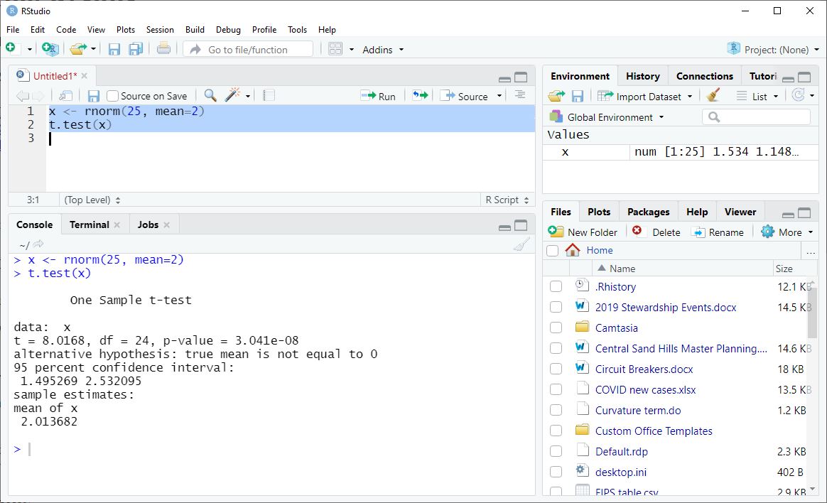
We can use the output of a t-test as an example.
    x <- rnorm(25, mean=2)
    t.test(x)
You can resize your Console pane to see more (or less) of your output at once. The width of your Console affects where the lines of print output break, so adjust this before you run your commands.
The Console is a “buffer” that only holds 1000 lines of output. With a huge amount of output you cannot scroll back to the beginning. We will later deal with this by saving output automatically.
1.2.2 Graphs
Graphs appear in the Plots pane, in the lower right of the RStudio workspace.
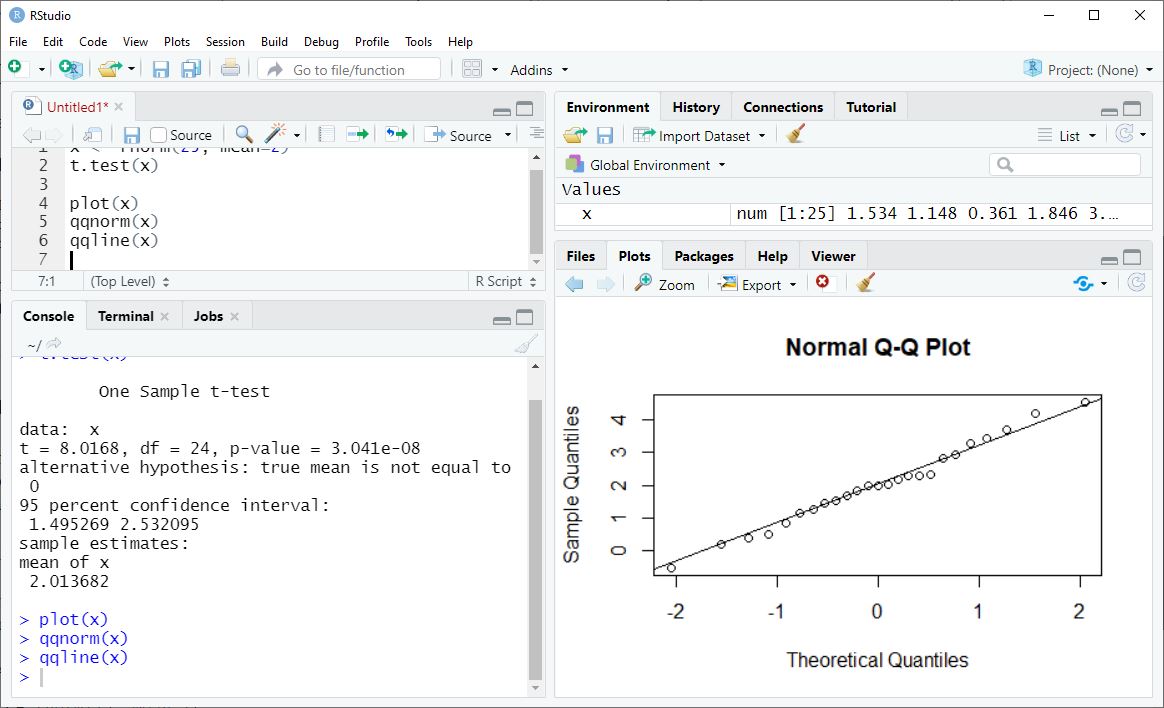
Plot the data from our last exercise as an example. The following three statements produce two plots.
    plot(x)
    qqnorm(x)
    qqline(x)
Like the Console, the Plots pane can be resized. This changes the look of the plot (the size and the aspect ratio). You can also pop a graph into a separate window with the Zoom button in the Plots toolbar.
If you have created more than one graph, you can use the left and right arrows in the Plots toolbar to scroll among your graphs.
1.2.3 Examining Data
Looking at data values is a little more complicated, because data comes in many forms in R. We will discuss the varieties of R data in more depth later, but for now there are three main strategies for examining data values and properties: the Environment pane, printing data to the Console, and viewing data frames and lists.
1.2.3.1 Environment Pane
The Environment pane in the upper right of the RStudio workspace shows the names of any data objects currently available in your computer’s memory.
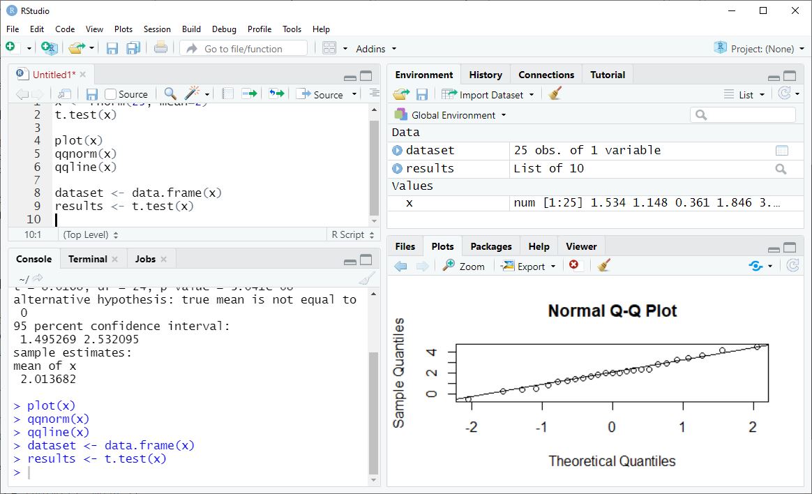
As examples, let’s save our
xdata as a data frame, and also save ourt.test()results as data.
    x <- rnorm(25, mean=2)
    dataset <- data.frame(x)
    results <- t.test(x)
In the Environment pane we see that x is a numeric vector (“num”) with
25 observations (“[1:25]”), and we can see a few
of the data values. For more complicated objects like dataset and results, we
can click on the blue arrow next to the name to see more details of what is inside
each object, including some data values. The main thing we get
out of the Environment pane is metadata, information about how
each data object is defined.
1.2.3.2 Viewing Data Frames and Lists
If you click on the name of a data frame or list object in the Environment pane, a window opens in the Script area of RStudio. For a data frame this gives you a spreadsheet-like view of the data values. For a list, it gives you a somewhat cleaner way to browse the metadata.
1.2.3.3 Printing Data
For basic data objects, printing them will show you the data values. To see just
a few of the data values, use the head() or tail() functions.
head(x)[1] 1.9995955 3.3253008 1.2070245 2.9545859 0.7674088 2.1404606tail(dataset) x
20 1.547199798
21 3.077790631
22 -0.006397434
23 1.687482573
24 2.185901053
25 2.943361027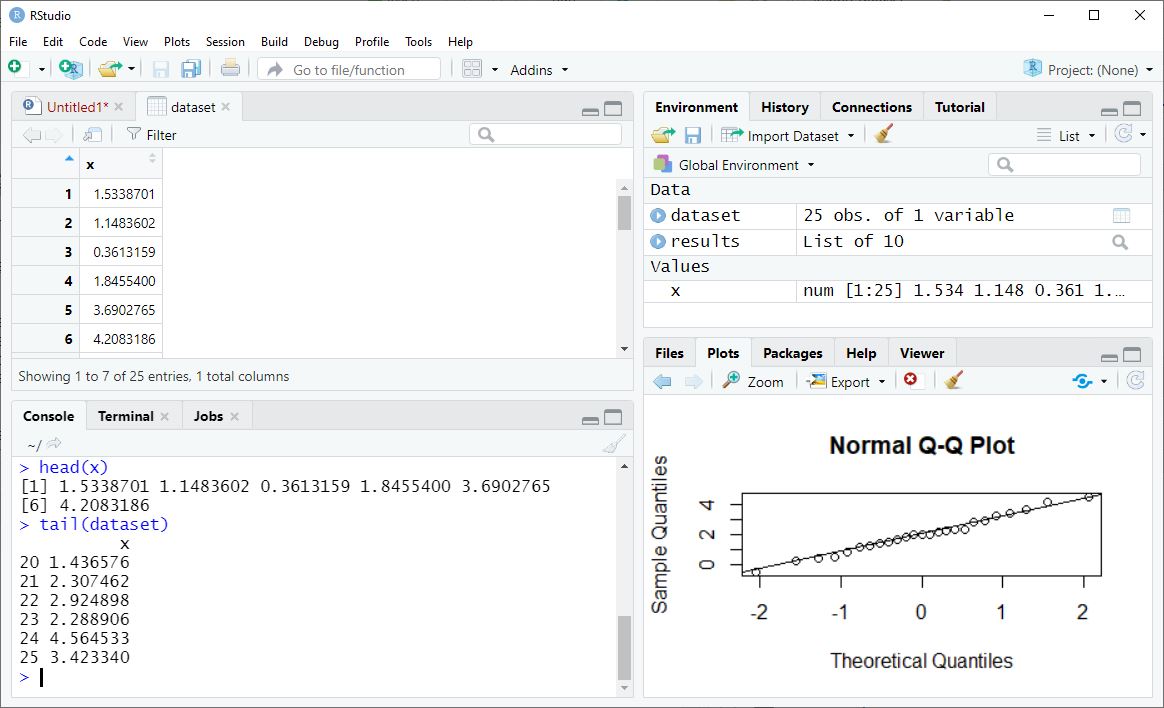
How an object is printed depends on its class. So printing a data object
like results does not just show the data elements it stores.
To see the actual data values being stored typically requires extracting
or coercing the data object to print the elementary
data values – topics for later.
If we strip away the class of results R just prints the
data it contains without interpretation and we get something
quite different from the earlier print output!
class(results) <- NULL
results
$statistic
t
10.5227
$parameter
df
24
$p.value
[1] 1.800661e-10
$conf.int
[1] 1.618880 2.408875
attr(,"conf.level")
[1] 0.95
$estimate
mean of x
2.013878
$null.value
mean
0
$stderr
[1] 0.1913842
$alternative
[1] "two.sided"
$method
[1] "One Sample t-test"
$data.name
[1] "x"1.3 Saving Commands and Results
Like most statistical software, you save the pieces of an R project in several different files.
1.3.1 Scripts
Scripts and your data are the most important pieces of any project. With good scripts and your original data, your work is documented and reproducible.
You save scripts pretty much the way you would expect. With the script editor as the active window, click File - Save As and give your file a name, along with the file extension “.r”. Although this is just a plain text file, the “.r” file extension will ensure that the software and the operating system recognize this as an R script, enabling the software to work with the file more gracefully.
You can open previously saved scripts from the Files pane (lower right, tabbed with Plots). Just click on the file name.
When you shut down RStudio, any open scripts are automatically stored by default, and reappear when you start up RStudio again. However, they are not available outside of RStudio until you save them.
1.3.2 Data
Save the original data file(s) you started from. Often this will be a text or csv (comma-separated values) file.
Having read your data into R, cleaned it, and created any other data objects (including results objects), you may want to save your intermediate data. This is especially useful if data wrangling or modeling takes a lot of computer time to run.
You will seldom save your entire Global Environment (the data objects listed in the Environment pane). On those rare occasions when you need to – you have a bus to catch, or the fire alarm has gone off – click on the Save icon on the Environment toolbar, and give your data file a name - RStudio automatically appends an “.RData” file extension for you.
Reload saved data by clicking on the file name in the Files pane, or by clicking on the Open icon on the Environment toolbar.
Finally, saving specific data objects can be automated by including the appropriate
statements in your scripts, save() or save.image().
1.3.3 Plots
You save plots pretty much as you expect. In the Plots pane, click on Export - Save as Image … on the toolbar. Pick an appropriate image format. The options depend on your computer’s operating system. Which format you want depends on how you intend to use the saved image. Then give the file a name.
This can also be automated with scripted commands. See help(Devices).
You won’t be able to reopen saved graphics within RStudio.
1.3.4 Text
Surprisingly, RStudio does not make it simple for you to save the contents of the Console. The general idea is that you are usually better off automatically saving your results, and this requires either batch processing (running your script in batch mode) or including some code in your script. We will go more into this in the next chapter.
Keep in mind, too, that the Console is limited to the last 1000 lines of text you output. If you have been working for a long period of time, or if you accidentally print a lot of data, your first results disappear and can only be recovered by rerunning your commands.
However, the quick-and-dirty method of saving the Console is to copy-and-paste it into a text file.
- In the Console, select the text you want to save. To save everything, right-click to bring up a context menu, then Select All.
- Key Ctrl-c to copy
- On the main menu, click File - Text File to open a blank file in the script editor. Then click within the blank editor.
- Key Ctrl-v to paste in the blank editor.
- Save the file. A file extension of “.txt” or “.log” is usually a good choice.
These can be reopened later from the Files pane.
To automate saving text output, see sink() or capture.output(). More
is in Saving R Output Automatically.
1.3.5 Exercises - Saving Files
- Save the following statements as a script. Run the statements and save the (print) output in a text file.
  x <- rnorm(20, mean=3, sd=3)
t.test(x)- The following statements perform an independent samples t-test. Save
these as a script, then run the commands and save the output. (They
make use of the R example data set,
mtcars.)
  data(mtcars)
t.test(mpg ~ am, data=mtcars)- (Extra credit) The results in exercise 2 are NOT a classic t-test.
Here, the variances of the two groups are not assumed to be equal.
Can you figure out how to run the classic test? If so, set that
up as a script and save the script and output. (Hint: See
help(t.test).)