SPSS Statistics for Students: Statistics and Graphs
IBM SPSS Statistics is software for managing data and calculating a wide variety of statistics. This document is intended for students taking classes that use SPSS Statistics. Those who plan on doing more involved research projects using SPSS should attend our workshop series.
If you are not already familiar with the SPSS windows (the Data Editor, Output Viewer, and Syntax Editor), please read SPSS Statistics for Students: The Basics.
Contents:
- Frequencies: Counts and Percents
- Descriptives: Means and Standard Deviations
- Histograms
- Crosstabs: Counts by Group
- Means by Group
- Bar Charts and Boxplots
- Correlation
- Scatterplots
- Hypothesis Testing
- Regression
- Learning More
The examples that follow are based on the sample data in
C:\Program Files\IBM\SPSS\Statistics\19\Samples\English\Employee data.sav
Frequencies: Counts and Percents
Counts and percents are wonderful statistics because they are easy to explain and quickly grasped. Frequencies also form the very foundation of most explanations of probability. They are an excellent place to begin understanding any data you may work with.
Menu and Dialog Box:
Analyze -> Descriptive Statistics -> Frequencies
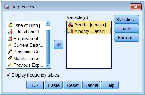
Select one or more variables in the selection list on the left, and move them into the analysis list on the right by clicking on the arrow in between. Then click OK.
Syntax:
frequencies variables = gender minority.
Output:
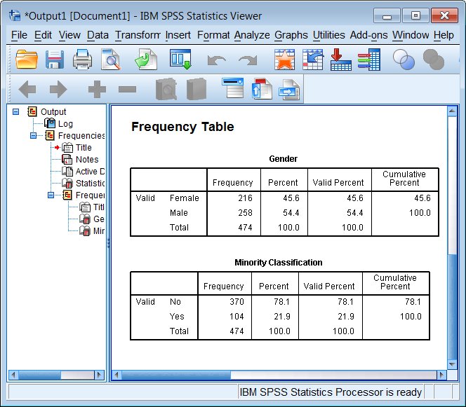
Note that this is one of the few instances where missing values (whether system missing . or user designated missing) show up in the default output table (however, not in this particular example).
Descriptives: Means and Standard Deviations
The mean and standard deviation of a variable are such fundamental quantities in statistics, that there are many SPSS commands that will report them to you. The most straightforward command to use is Descriptives.
Two other useful commands are Frequencies (in the dialog box, click on the Statistics button), when you want to see counts as well as means and standard deviations (perhaps for Likert scales), and Explore, which gives you such additional statistics as the median and interquartile range as well as a variety of graphs.
Menu and Dialog Box:
Analyze -> Descriptive Statistics -> Descriptives
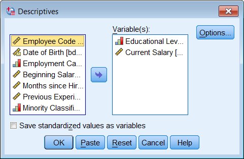
Select one or more variables in the selection list on the left, and move them into the analysis list on the right by clicking on the arrow in between. Then click OK.
Syntax:
descriptives variables=educ salary.
Output:
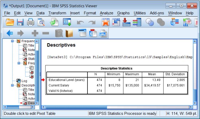
Histograms
SPSS has three different sets of commands for producing graphs. The easiest to learn and use are the oldest “legacy” graphing commands. They give you graphs with a default visual style (colors used, weight of lines, size of type, etc) that can be customized by hand.
Histograms are vexing because they can be alternately informative or deceptive, depending upon how the bins (the bar boundaries) are chosen. They are useful and popular because they are conceptually very simple, easy to draw and interpret, and if drawn well they can give a good visual representation of the distribution of values of a variable.
Menu and Dialog Box:
Graphs -> Legacy Dialogs -> Histogram
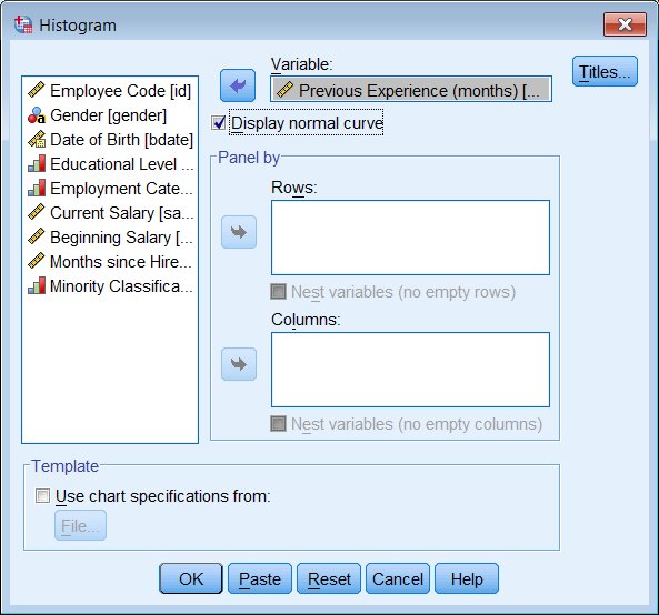
The basic histogram command works with one variable at a time, so pick one variable from the selection list on the left and move it into the Variable box. (A useful option if you expect your variable to have a normal distribution is to Display normal curve.)
Syntax:
graph /histogram(normal) = prevexp.
Output:

In this example, the distribution of the data is nothing like a normal distribution!
To edit colors, titles, scales, etc. double-click on the graph in the Output Viewer, then double-click on the graph element you want to change.
Crosstabs: Counts by Group
The basic crosstabs command just gives you counts by default. Typically it is useful to also look at either row-percents or column-percents, which must be specified as options.
Menu and Dialog Box:
Analyze -> Descriptive Statistics -> Crosstabs
Select one variable as the rows, another variable as the columns. Conventionally you might put an independent variable in the rows and a dependent variable in the columns, although mathematically it doesn't really matter. To get percents in your output, click on the Cells button and specify the kind of percents you want to see.
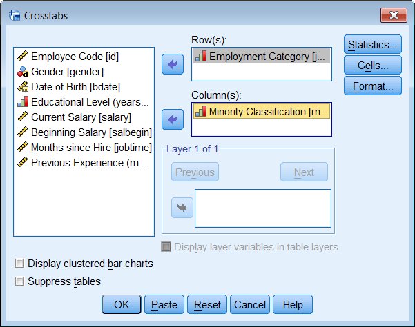
Syntax:
crosstabs
/tables=jobcat by minority
/cells=count row.
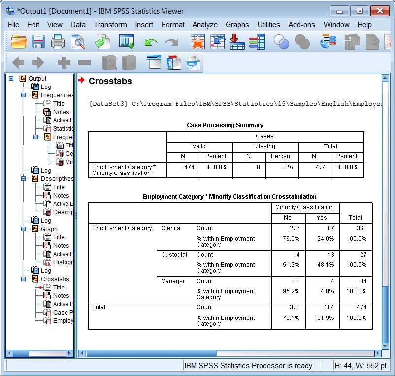
In this command syntax (and the next one, means), you see the key word by used to specify a categorical variable that divides the data into groups.
Output:
Means by Group
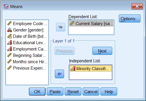
Menu and Dialog Box:
Analyze -> Compare Means -> Means
Select the variable(s) that you want means of, and move it to the Dependent List. Select the variable that divides the data into subsets (the “grouping” or “by” variable) and move it to the Independent List. You may have more than one variable in either/both list, and SPSS processes them in pairs and produces separate tables.
Syntax:
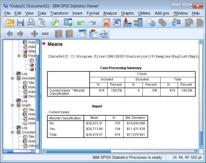
means tables=salary by minority.
Output:
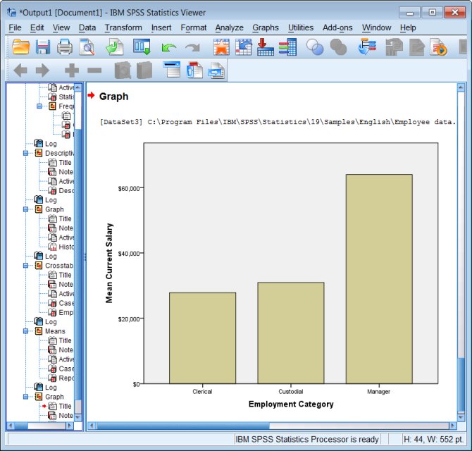
Bar Charts
Similar to a histogram, the x axis is treated as a categorical variable, and the y axis represents one of a variety of summary statistics: counts (a.k.a. a histogram!), means, sums, etc.
Menu and Dialog Box:
Graphs -> Legacy Dialogs -> Bar
This takes you through an initial dialog box, where you choose among several basic schemas for making bar charts,
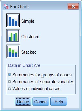
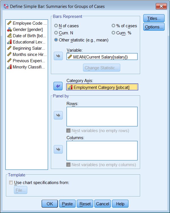
and then to the main dialog box. To graph means by groups, select Other statistic for what the bars represent, the variable for which you want to calculate means in the Variable box (means will be the default statistic), and the group in the Category Axis box.
Syntax:
graph /bar=mean(salary) by jobcat.
Output:
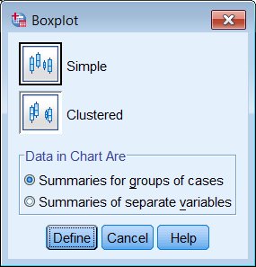
Boxplots
Menu and Dialog Box:
Graphs -> Legacy Dialogs -> Boxplot
As with bar charts, you first choose a specific boxplot schema from an initial dialog box,
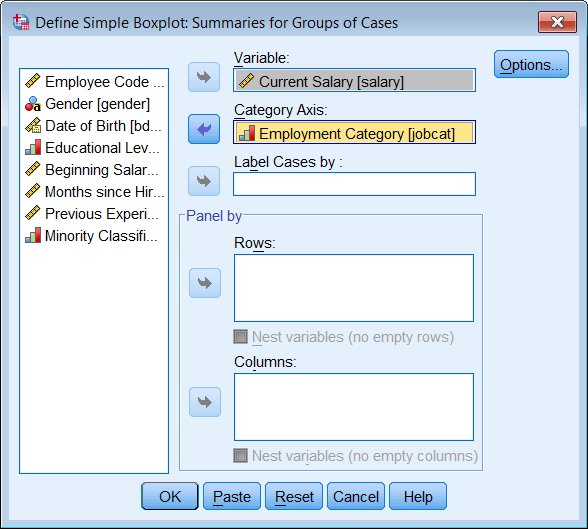
and then choose the analytical variable (the one you want to see medians and interquartile ranges for, the y axis), and the categorical variable (the x axis).
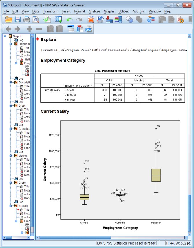
Syntax:
examine variables=salary by jobcat
/plot=boxplot
/statistics=none
/nototal.
Output:
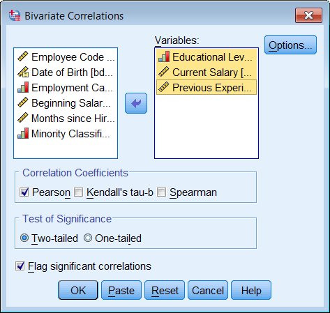
Correlation
Menu and Dialog Box:
Analyze -> Correlate -> Bivariate
SPSS calculates bivariate correlations (the Pearson’s r) for all pairs of variables in the list.
Syntax:
correlations /variables=educ salary prevexp.
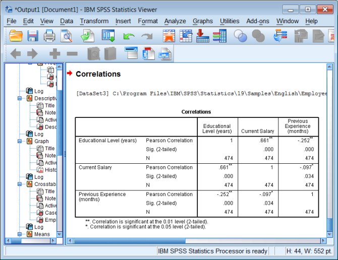
Output:
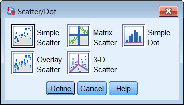
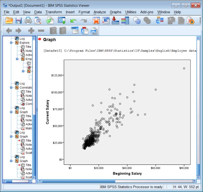
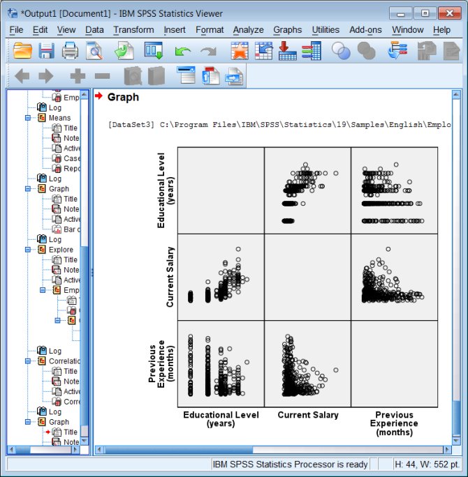
Scatter Plots
Both simple scatter plots and scatter plot matrixes are pretty easy to produce.
Menu and Dialog Box:
Graphs -> Legacy Dialogs -> Scatter/Dot
Takes you through two dialog boxes. First you choose the scatter plot schema you want to work with,
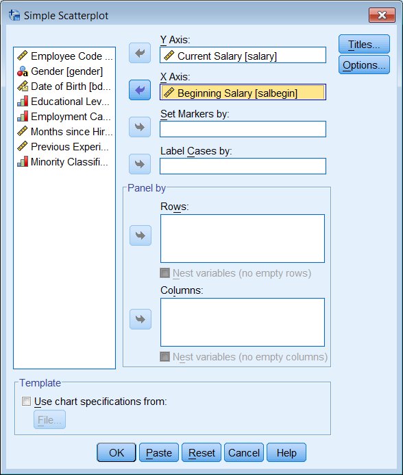
And then you specify the variables with the x and y coordinates of the points you wish to plot.
Syntax:
graph /scatterplot=salary with salbegin.
graph /scatterplot(matrix)=salary salbegin prevexp.
Output:
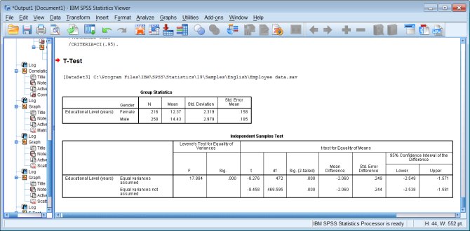
T-tests
T-test can be used in a variety of ways, and SPSS gives you quick access to three of them (univariate, grouped, and paired) through the Compare Means menu. They all access the same t-test command.
Menu and Dialog Box:
Analyze -> Compare Means -> Independent-Samples T Test
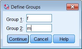
When setting up an independent-samples (grouped) t-test, you not only specify the variable being tested and the grouping variable, but you also have to specify which data values represent the two groups you want compared (because in general the grouping variable might have an arbitrary number of categories, not just two). Use the Define Groups button, and type in the data values (not the value labels) that define the groups being compared.
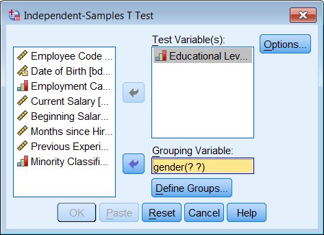
If you type in an invalid data value for any of the groups, SPSS will not catch your mistake until you actually run the command. You need to know what your data look like before you get to this dialog box, because SPSS will not let you browse your data set while a dialog box is open.
Syntax:
t-test groups=gender('f' 'm')
/variables=educ.
Output:
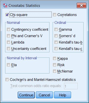
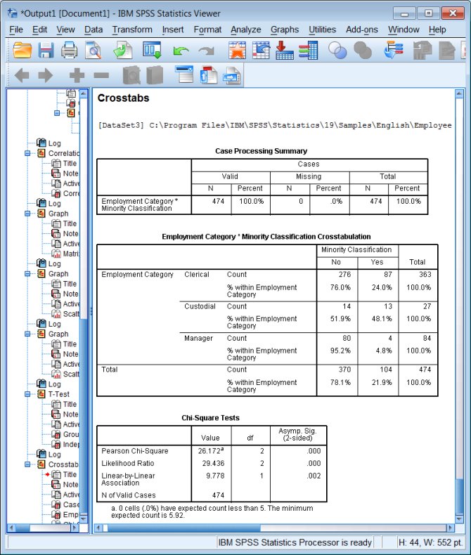
Chi-square Tests
Like t-tests, chi-square tests come up in a wide variety of circumstances, the most common of which is assessing the independence of two variables in a contingency table (a crosstab). So this chi-square test is specified as an option on a crosstab command.
Menu and Dialog Box:
Analyze -> Descriptive Statistics -> Crosstabs
In the main dialog box, click on the Statistics button, then select Chi-square and Continue back to the main dialog box. Specify your variables and run.
Syntax:
crosstabs
/tables=jobcat by minority
/statistics=chisq
/cells=count row.
Output:
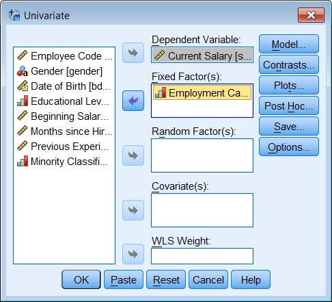
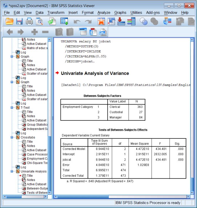
ANOVA Tables and Tests
ANOVA tables are a core concept in statistics, and they are produced by several different commands in SPSS, including oneway, glm, and unianova. The unianova command is perhaps the easiest to use overall, because it allows you to use string (character) variables as factors.
(If you are doing a one-way ANOVA and your factor is coded in numeric form, then oneway is even easier to use.)
Menu and Dialog Box:
Analyze -> General Linear Model -> Univariate
For a simple ANOVA, your factors are considered Fixed Factors. If you have more than one factor and you do not want to include interactions in your model, you will need to specify that with the Model button.
Syntax:
unianova salary by jobcat.
Output:
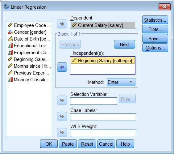
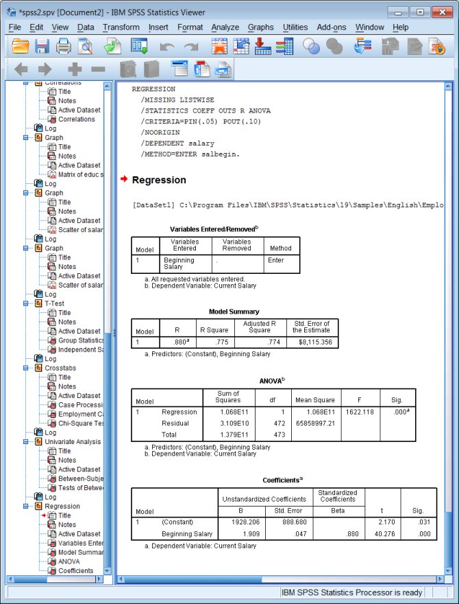
Regression
Menu and Dialog Box:
Analyze -> Regression -> Linear
Syntax:
regression
/dependent salary
/method=enter salbegin.
Output:
Learning More
To learn more about how to use the SPSS windows, you can look at the on-line tutorial that comes with the software: click Help, Tutorial.
To learn more about specific data management or statistical tasks, you should try the on-line Help files. Click Help, Topics and you can read about a variety of basic SPSS topics, or search the index.
Your instructor and/or TA are your best resource for class-specific tasks.
Doug Hemken, a statistical computing specialist for the SSCC, is available to help students at UW-Madison with homework and class projects. His hours are 10AM-2PM Monday-Friday or by appointment in 4226I Sewell Social Sciences Building. If he is not available, other SSCC staff may be able to assist you: go to 4226 and then look for the red “Stat Consultant” or the yellow “SSCC Consultant” sign.
Last Revised: 3/29/2010