R for Researchers: Regression (GLM) solutions
April 2015
This article contains solutions to exercises for an article in the series R for Researchers. For a list of topics covered by this series, see the Introduction article. If you're new to R we highly recommend reading the articles in order.
There is often more than one approach to the exercises. Do not be concerned if your approach is different than the solution provided.
The following preparation code was used to prepare the R session for these solutions
#######################################################
#######################################################
##
##   Environment Setup
##
#######################################################
#######################################################

library(faraway)      # glm support
library(MASS)         # negative binomial support
library(car)          # regression functions
library(lme4)         # random effects
library(ggplot2)      # plotting commands
library(reshape2)     # wide to tall reshaping
library(xtable)       # nice table formatting
library(knitr)        # kable table formatting
library(grid)         # units function for ggplot

saveDir <- getwd()    # get the current working directory

wd <- "u:/RFR"        # path to my project
setwd(wd)             # set this path as my work directory
Exercise solutions
Use the following code to load the warpbreaks data set and examine the variables in the data set.
data(warpbreaks)

str(warpbreaks)
'data.frame': 54 obs. of 3 variables: $ breaks : num 26 30 54 25 70 52 51 26 67 18 ... $ wool : Factor w/ 2 levels "A","B": 1 1 1 1 1 1 1 1 1 1 ... $ tension: Factor w/ 3 levels "L","M","H": 1 1 1 1 1 1 1 1 1 2 ...plot(warpbreaks)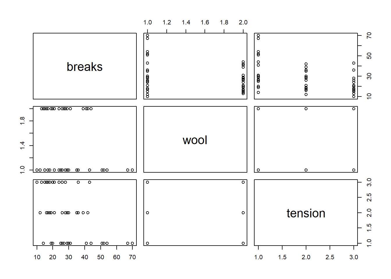
Use the poisson family and fit breaks with wool, tension, and their interaction.
pMod <- glm(breaks~wool*tension,family=poisson, data=warpbreaks)
summary(pMod)
Call: glm(formula = breaks ~ wool * tension, family = poisson, data = warpbreaks) Deviance Residuals: Min 1Q Median 3Q Max -3.3383 -1.4844 -0.1291 1.1725 3.5153 Coefficients: Estimate Std. Error z value Pr(>|z|) (Intercept) 3.79674 0.04994 76.030 < 2e-16 *** woolB -0.45663 0.08019 -5.694 1.24e-08 *** tensionM -0.61868 0.08440 -7.330 2.30e-13 *** tensionH -0.59580 0.08378 -7.112 1.15e-12 *** woolB:tensionM 0.63818 0.12215 5.224 1.75e-07 *** woolB:tensionH 0.18836 0.12990 1.450 0.147 --- Signif. codes: 0 '***' 0.001 '**' 0.01 '*' 0.05 '.' 0.1 ' ' 1 (Dispersion parameter for poisson family taken to be 1) Null deviance: 297.37 on 53 degrees of freedom Residual deviance: 182.31 on 48 degrees of freedom AIC: 468.97 Number of Fisher Scoring iterations: 4Check to see if this is an appropriate model. If not, choose a more appropriate model form.
1 - pchisq(deviance(pMod),df.residual(pMod))[1] 0pMod2 <- glm(breaks~wool*tension, family="quasipoisson", data=warpbreaks) pMod2Diag <- data.frame(warpbreaks, link=predict(pMod2, type="link"), fit=predict(pMod2, type="response"), pearson=residuals(pMod2,type="pearson"), resid=residuals(pMod2,type="response"), residSqr=residuals(pMod2,type="response")^2 ) ggplot(data=pMod2Diag, aes(x=fit, y=residSqr)) + geom_point() + geom_abline(intercept = 0, slope = 1) + geom_abline(intercept = 0, slope = summary(pMod2)$dispersion, color="green") + stat_smooth(method="loess", se = FALSE) + theme_bw()`geom_smooth()` using formula 'y ~ x'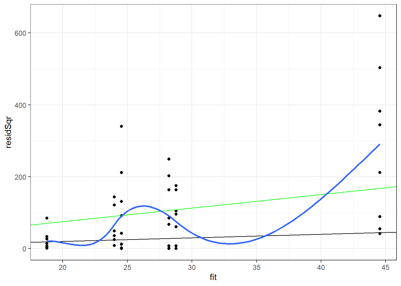
nbMod <- glm.nb(breaks~wool*tension,
                data=warpbreaks)
summary(nbMod)
Call: glm.nb(formula = breaks ~ wool * tension, data = warpbreaks, init.theta = 12.08216462, link = log) Deviance Residuals: Min 1Q Median 3Q Max -2.09611 -0.89383 -0.07212 0.65270 1.80646 Coefficients: Estimate Std. Error z value Pr(>|z|) (Intercept) 3.7967 0.1081 35.116 < 2e-16 *** woolB -0.4566 0.1576 -2.898 0.003753 ** tensionM -0.6187 0.1597 -3.873 0.000107 *** tensionH -0.5958 0.1594 -3.738 0.000186 *** woolB:tensionM 0.6382 0.2274 2.807 0.005008 ** woolB:tensionH 0.1884 0.2316 0.813 0.416123 --- Signif. codes: 0 '***' 0.001 '**' 0.01 '*' 0.05 '.' 0.1 ' ' 1 (Dispersion parameter for Negative Binomial(12.0822) family taken to be 1) Null deviance: 86.759 on 53 degrees of freedom Residual deviance: 53.506 on 48 degrees of freedom AIC: 405.12 Number of Fisher Scoring iterations: 1 Theta: 12.08 Std. Err.: 3.30 2 x log-likelihood: -391.125Use the backward selection method to reduce your model, if possible. Use your model from the prior problem as the starting model.
step(nbMod, test="LRT")Start: AIC=403.12 breaks ~ wool * tension Df Deviance AIC LRT Pr(>Chi) <none> 53.506 403.12 - wool:tension 2 61.712 407.33 8.206 0.01652 * --- Signif. codes: 0 '***' 0.001 '**' 0.01 '*' 0.05 '.' 0.1 ' ' 1Call: glm.nb(formula = breaks ~ wool * tension, data = warpbreaks, init.theta = 12.08216462, link = log) Coefficients: (Intercept) woolB tensionM tensionH woolB:tensionM 3.7967 -0.4566 -0.6187 -0.5958 0.6382 woolB:tensionH 0.1884 Degrees of Freedom: 53 Total (i.e. Null); 48 Residual Null Deviance: 86.76 Residual Deviance: 53.51 AIC: 405.1No terms can be dropped from the model.
Check the residual variance assumption for your model.
nbModDiag <- data.frame(warpbreaks,
                        link=predict(nbMod, type="link"),
                        fit=predict(nbMod, type="response"),
                        pearson=residuals(nbMod,type="pearson"),
                        resid=residuals(nbMod,type="response"),
                        residSqr=residuals(nbMod,type="response")^2
                        )

ggplot(data=nbModDiag, aes(x=fit, y=residSqr)) +
  geom_point() +
  geom_abline(intercept = 0, slope = 1) +
  geom_abline(intercept = 0, slope = summary(pMod2)$dispersion,
              color="green") +
  stat_function(fun=function(fit){fit + fit^2/summary(nbMod)$theta},
                color="red") +
  stat_smooth(method="loess", se = FALSE) +
  theme_bw()
`geom_smooth()` using formula 'y ~ x'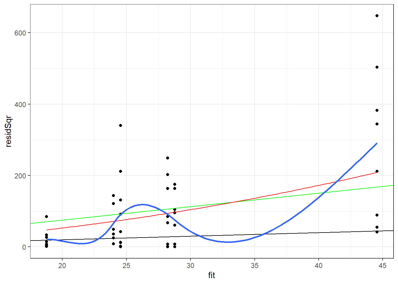
The negative binomial model is closer to means of the loess line than to the quasipoisson model. The range of values predicted by the model for the predicted values below 20 appears to be overstated by this model, though not as much as by the quasipossion model.
Return to the Regression (OLS) article.
Last Revised: 3/4/2015