R for Researchers: R Markdown
April 2015
This article is part of the R for Researchers series. For a list of topics covered by this series, see the Introduction article. If you're new to R we highly recommend reading the articles in order.
Overview
This article will introduce you to R Markdown, a document writing program, and demonstrates using RStudio's Git diff, a tool to examine when prior changes were made to a project. These tools are part of RStudio's development environment. They help you work more efficiently.
R Markdown has two advantages that are of interest to a researcher. The first is it allows the results of R code to be directly inserted into formatted documents. The second advantage is it is incredibly easy to use. This ease is a result of R Markdown only using a small set of features and this reduces the complexity of the needed commands. This set of features supports the most commonly used formatting, resulting in the ability to create most documents. These features make R Markdown documents easy to write and the process less error prone.
Git diff allows you to look at what has changed in a file, or files, between any two saved project states. This can be very helpful in determining why results have changed.
Preliminaries
You will get the most from this article if you follow along with the examples in RStudio. Working the exercise will further enhance your skills with the material. The following steps will prepare your RStudio session to run this article's examples.
- Start RStudio and open your RFR project.
- Confirm that RFR (the name of your project) is displayed in the upper left corner of the RStudio window.
- Confirm that there is a Git tab in one of the tab panes.
Files types
RStudio is able to work with a variety of programming languages. This article series covers two of these program languages, R and R Markdown. This article provides an introduction to R Markdown files, which have a file type of .Rmd. R Programs are called R scripts, which have file type .R. The next article introduces R Scripts.
This article series will use .txt and .csv files for datasets. These are the common file types used to import text datasets. The use of these file types will be covered in the data preparation article. This article series will not make use of R's dedicated data file type for data, .RData.
Markdown and R Markdown
Markdown is a tool used to create formatted documents. Markdown source files, file type .md, contain text and formatting commands. Markdown's formatting commands are simpler than most other formatting languages, such as LaTeX or HTML, because it has a smaller number of features. This small set of features supports the most commonly used formatting. The source files are also easier to read than LaTeX or HTML. Markdown is a good choice to format most documents.
R Markdown is an extension of Markdown. R Markdown adds a few features which include R code and results in the formatted document. This allow you write documents which integrate results from your analysis. Incorporating R results directly into your documents is an important step in reproducible research. Any changes that occur in either your data set or the analysis are automatically updated in your document the next time the document is created. There is no more going back through documents trying to find every thing that needs to be fixed when an analysis is rerun. This results in not only greater efficiency, but also fewer errors in documents.
RStudio creates a document, this is called knitting, from an .Rmd file in two steps. In the first step, the R commands are run. The results of the R commands are incorporated with the text and Markdown commands from the .Rmd file. The result of the first step is a .md file. The second step uses the Markdown formatting commands to format the final document. These steps are done together for you by simply pushing the knit button in RStudio.
R Markdown files can be knit to html, pdf, or Word documents. The knitted documents should not be changed by hand. Any edits that are made by hand will be lost when the document is knit again. We do not recommend knitting to Word, because a Word document is a form that is tempting to edit. We recommend knitting to either pdf or HTML files. Programs to read .html and .pdf files are widely available at no cost. In this article series we will generate HTML files.
Writing R Markdown documents is a little different process than with "What You See Is What You Get" (WYSIWYG) editors, such as Microsoft Word. The examples and exercises in this article series are designed to give you the practice and experience needed to be comfortable with this type of document creation process. As you start working with R Markdown, you may find it convenient to knit your document often. As you gain experience with R Markdown, you will knit much less frequently.
Creating an R Markdown file
To start a document we need to create a new R Markdown file.
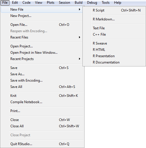
From the File menu, select New File and then R Markdown from the drop down menus.
IDE New File
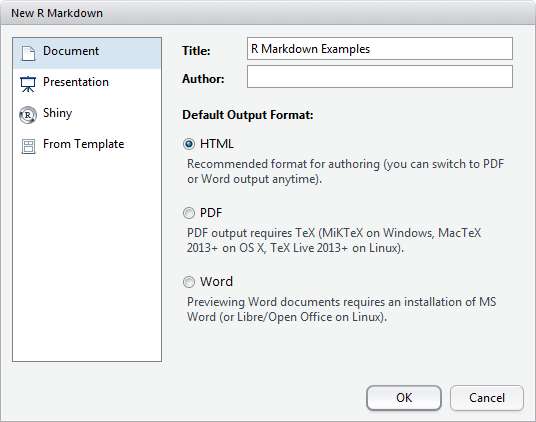
A New R Markdown window will open. Enter a title, here we will use "R Markdown Examples". This is the title which will be displayed in the document and is not the name of the file.
IDE New File
Click the OK button in the New R Markdown window.
This new R Markdown file is now open in RStudio. The file has not been named or saved. Click the save icon, which looks like a floppy disk, in the source pane.
A Save File window will open. Since we are in a project, RStudio sets the folder to the project folder. If you want the file saved in another folder, such as a sub folder of the project, you navigate to the desired folder. We will use the default of the project folder. Enter the name of the file, here we will use "RmdExamples". Click the Save button.
In the Git tab you can see that the Git status of RmdExamples.Rmd has not been established. That is because we have not either added this file to the Git repository or told Git to ignore it. We will commit this file after we have modified it.
Exercises
Open a new R Markdown file with an output format of HTML. Give the document the title "My RFR class notes".
Save the file created in exercise 1 as "Notes" in the RFR project folder.
File tab
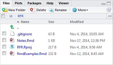
Notice in the Files tab that the files RmdExamples.Rmd and Notes.Rmd are now seen in the the RFR project folder.
If the Files tab is not displayed, click on the tab labeled Files.
IDE File tab
The File tab can be used to open and move files similarly to the Windows Explorer window in the Microsoft Windows environment. If subfolders are added to the project folder, navigating to these folders is also the same as in Windows.
Text formatting using Markdown syntax
Markdown files can be written using any plain text editor such as notepad. We will write our Markdown files using RStudio's editor.
R Markdown files start with a set of lines which begin with --- on a line and end similarly with a line containing --- . This set of lines between and including the lines with ---, is called the metadata section. Markdown commands and text will be added after the metadata section. The RmdExamples file, which is opened in the source pane, has the following metadata section.
---
title: "R Markdown Examples"
output: html_document
---
This article series will not change or edit the metadata section. For more information on the metadata section see html metadata section and pdf metadata section.
Markdown uses #, *, blank lines, and indented lines for the most common formatting commands. This makes Markdown documents easy to type and makes it easy to read the unformatted document. We will look at a simple example as an introduction to the Markdown syntax.
Let's say we wish to create a document with an introductory paragraph followed by a sub header, another paragraph, and finally a list.
The following Markdown source text is one way to write this example.
  Introductory paragraph text.

  #### Sub header text

  Another paragraph text.

  1. List item one text
  2. List item two text
The above Markdown produces the following in the knitted document.
Introductory paragraph text.
#### Sub header text
Another paragraph text.
- List item one text
- List item two text
- List item one text
This example uses just a few formatting commands. Blank lines indicate the end of a paragraph. Placing one to six # at the beginning of a line indicate what follows is a header with the header level being the number of # used. Starting a line with 1. starts a numbered list.
Run this example code in your RmdExample file.
- Delete all the lines which follow the metadata section in the RmdExample file.
- Copy the Markdown source text from the example above and paste the source text in the RmdExample file after the metadata section. It is best to leave at least one blank line after the metadata section before your code starts.
- Click on the knit button in the source pane.
- A viewer window will open with your example document displayed. Your viewer should display the title of the document, which is "R Markdown Examples" here. Following the title should be the text formatted similarly to what is shown above. Note there will be some differences in formatting due to the styles associated with the web site of this article.
Now that we have made some changes to the RmdExamples file, we will do some source control work.
Add RmdExamples.html to gitignore. Remember this is done by selecting RmdExamples.html in the Git tab and then selecting Ignore from the tools drop down menu.
Stage RmdExamples.Rmd and gitignore. Remember this is done by clicking the staged box in front of each file in the Git tab.
Commit the files with the commit message "Added Markdown examples". Remember this is done by clicking the commit icon in the Git tab and then entering the message in the Commit message box.
Close the Git commit and RStudio Review Changes windows
Markdown syntax
A paragraph is started and ended with a blank line before and after the paragraph text. There can be no blank line within the text of a paragraph. Alternately, the end of a paragraph can be indicated with two blank spaces at the end of a line of text.
There are six header levels. The number of # determines the header level. A blank line is required prior to the line which starts a header. Examples of headers one through three are shown below. Note the formatting in your document may be slightly different due to the styles applied to this web site.
Header examples
# header 1results in
# header 1
## header 2results in
## header 2
### header 3results in
### header 3
There are several font modifications which can be used in your documents. The number of "*"s are used to determine italic and bold fonts. These font modifications are shown in the following example.
Font modification examples
*italic* **bold** ***bold and italic*** ~~strikethrough~~results in
italic bold bold and italic
strikethrough
There are two list types, enumerated and unordered. Unordered list items are identified with the * symbol at the beginning of a paragraph. This means there must be a blank before the list item or the prior line must end with two blank spaces. An enumerated list item is identified with an integer number followed by a period at the beginning of a paragraph. The first number of the list is the integer number provided for the first item in the list. The following items are numbered sequentially from the start number regardless of the number used to identify the subsequent enumerated items.
Unordered list example
  * unordered item
  * another unordered item
results in
- unordered item
- another unordered item
Enumerated list example, starting with number 1
  1. numbered item
  1. another numbered item
results in
- numbered item
- another numbered item
- numbered item
Text can be indented two ways depending on if the indent is within a list or not. Within a list, four spaces at the begin of the line indicates the text is to be indented one nesting level. Use four additional spaces for each additional nesting level. To indent text which is not in a list, use a block quote. This is done by starting a line with four spaces.
Indented text example
Indenting a block quote
indented textresults in
indented text
Indenting a text within a list
  * List item
      indented text
results in
- List item
indented text
- List item
Links to other documents make use of [] for the displayed text and () for the path to the document.
link example
[link text](link path)results in
Information on additional Markdown formatting commands can be found at Markdown Basics.
Exercises
These exercises are to be done in the Notes.Rmd file that you created above.
Remove all of the document text and commands after the metadata section.
Add a level 2 header with the title of this article.
Following the header created in the exercise above, write a note to remind yourself of at least one thing about formatting using Markdown.
In the text you wrote for the exercise above, use a text modifier (bold, italic, etc.) to highlight a key work or phrase from the text.
Ignore the Notes.html file and commit the Notes.Rmd and .gitignore files with the commit message "Added notes for R Markdown article".
Mathematical equation formatting commands using LaTeX syntax
Mathematical expressions and equations can be formatted using LaTeX math formatting. LaTeX math formatting can be used for all three output formats, HTML, pdf, and Word documents. Information of formatting mathematics in LaTeX can be found at LaTeX/Mathematics.
HTML pages which include LaTeX formatting use mathjax and javascript for this formatting. Readers may be prompted to allow javascript to run when the webpage is opened.
The syntax to start and end LaTeX math formatting is done with either $ or $$.
LaTeX formatting examples
Inline LaTeX equation $y = 3 + 2x$results in
Inline LaTeX equation \(y = 3 + 2x\)
LaTeX equation $$y = 3 + 2x$$results in
LaTeX equation \[y = 3 + 2x\]
R code formatting commands using R Markdown syntax
R code can be included in a document as inline code or as a chunk. A code chunk is a block of code which is rendered in the document as a separate element in the document, not part of a paragraph of text. This may be a figure or a block of block of code and results. Inline R code displays only the text results of the R code in the document. The text returned by R will receive the same formatting as the text it is inline with (paragraph, header, etc.) Any graphics or other non-text results from inline code will not be included in the document.
We will look at a simple example as an introduction to including R code in R Markdown.
As an example, lets say we have a document which is to have the value of the constant \(e\) and a scatter plot.
The document text might be.
  #### Example of integrated R results

  This is inline code to produce the constant $e$, `r exp(1)`.

  This is an R chunk which produces a graph.

  ```{r }
  plot(1:10,(1:10+rnorm(10)) )
  ```
Add the lines above to your RmdExamples file. Add these new lines at the bottom of the file, after the lines for the Markdown example from above.
Knit RmdExamples document and you should see the following lines having been added to the HTML file.
#### Example of integrated R results
This is inline code to produce the constant \(e\), 2.7182818.
This is an R chunk which produces a graph.
plot(1:10,(1:10+rnorm(10)) )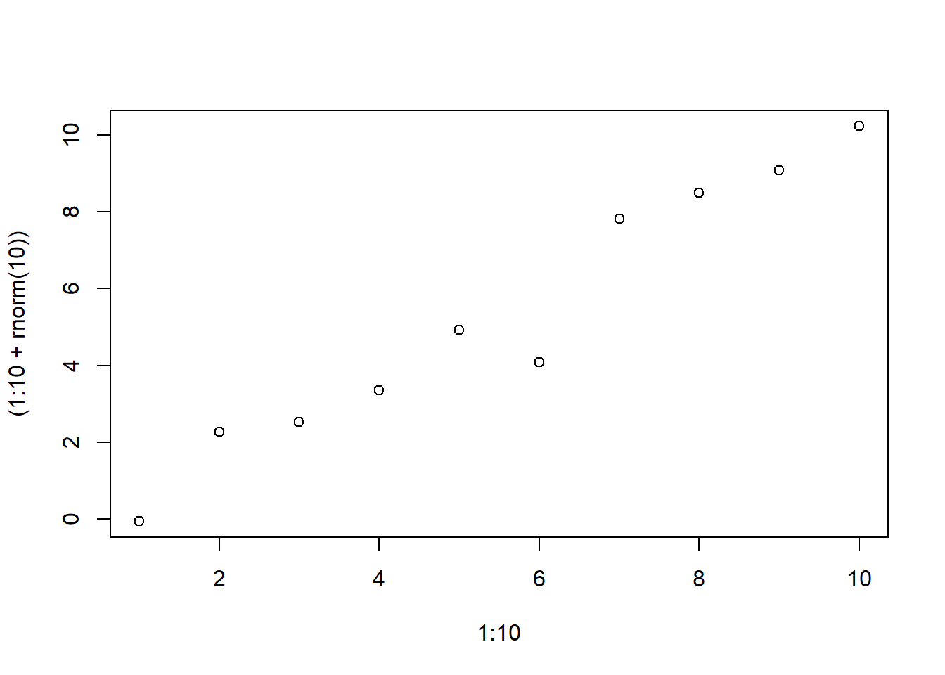
Commit the changes to RmdExmples.Rmd with the commit message of "Added R chunk example to RmdExamples".
R code syntax
Inline code is identified with a back tick (above the tab key on a keyboard) followed by r and ends with a back tick.
Example
$\pi$ = `r pi`results in
\(\pi\) = 3.1415927
Chunks start with ```{r name, options} and end with ```. The name is an optional identifier for the chunk and options allow for control of the execution and formatting of the R chunk and it's results.
Example
 \```{r \}
 pi
 ```
results in
pi## [1] 3.141593
Chunk options
Chunk options allow control over the display of both the source R code and R's results. The following is a list of some common chunk options. We will use most of these options in this article series.
- echo controls the display of the R source code. When set to FALSE, the R source code is not included in the document. The formatting of R's results is not affected by this option.
- comment controls what characters are displayed in front of R text results. When set to NA, no characters are displayed.
- results controls if text results are display and if they are formatted. When set to "hide", text results are not included in the document. When set to "asis", no formatting is done by knitr. This is useful for tables which have been formatted by R.
- message controls the display of messages. When set to FALSE, messages are not included in the document.
- warning controls the display of warning messages. When set to FALSE, warning messages are not included in the document.
- fig.show controls if graphics are displayed. When set to "hide", graphics are not included in the document.
- fig.align controls the horizontal position of graphics. When set to "center" results in the figure being centered. Left align is the default.
- out.height controls the height of the figure in the final document.
- out.width controls the width of the figure in the final document.
- fig.cap controls the caption which is displayed with a graphic. This is only supported for pdf documents. This is a result of RStudio using Pandoc to format the Markdown for pdf documents.
For a more complete discussion of code chunk options see Options:Chunk options.
The line which starts a chunk cannot be split into multiple lines. This results in some options list extending beyond the width of a line in your editor. This causes no issues for RStudio, though the R Markdown code is slightly less easy to read.
In most documents you will only want to see selected results from your R code. You will want the R code to run quietly in the background. Then you will use either inline or chunks to produce the selected results needed in the document. Chunk options allow for situations like this. The following example uses some made up results. We do not want to see the code which produced the results in the document. But we do want to include the results in the document.
The following is an example of R Markdown not displaying anything other than errors from a code block.
  ```{r, echo=FALSE, results='hide', message=FALSE, warning=FALSE, fig.show='hide'}
  # Made up results
  obs = 57
  pValue = .003
  ```

  #### Summary

  The test of `r obs` subjects resulted
  in a p-value of `r pValue `.
Produces the following two lines in a document.
#### Summary
The test of 57 subjects resulted in a p-value of 0.003.
Exercises
These exercises are to be done in the Notes.Rmd file that you created above. Add the work for these problems at the end of the file, after the work done for the previous exercises.
Demonstrate the use of in line R code to calculate the results of ((43 - 17)*.1)^2.
Demonstrate the use of a chunk to calculate the expression from the prior problem.
Same problem as prior problem with the addition of using chunk option(s) to prevent the R source code from being displayed.
Commit the Notes.Rmd file with the commit message "Added R code examples to Notes".
Git diff
One of the benefits of using Git for source control is its ability to display what has changed and when. This is done with a Git diff. A diff shows what has changed between any two project states. A project state is either a set of files as they were at a prior commit or the files as they are in the work directory. RStudio allows you to diff between adjacent project states. This is either the work directory to the last commit or any commit with the prior commit. To view diffs between other project states use a Git GUI such as SourceTree.
RStudio's Review Changes window is used to view the diffs. This is the same Review Changes window which we used in the Project's article when committing the .gitignore file and to view the project log. Clicking the diff icon in the Git tab opens the Review Changes window with the Changes view displayed. This view shows the diff between the work directory and the most recently committed files. This view was used in the Project's article when committing the .gitignore file. Clicking the history icon, which looks like a clock in the Git tab, opens the History view in the Review Changes window. This view shows the changes between any two adjacent commits. This view was used in the Project's article when we viewed the log. To switch between the Changes and History views use the Changes and History buttons in the upper left corner of the Review Changes window.
We have seen the diff of the work directory with each of the commit we have done. We will look at the diffs between adjacent commits for the RmdExample.Rmd file.
Click on the History icon in the Git tab.
The Review Changes window opens with the History view displayed.
In the log pane, top pane, in the Review Changes window, click on the "Added Markdown examples" commit.
The "Added Markdown examples" commit will be highlighted in log pane. In the review pane, lower pane, you will see the list of files which were committed. Below this list are the changes from the prior commit which were made to each of these files. The prior commit here is the "Initial commit" commit.
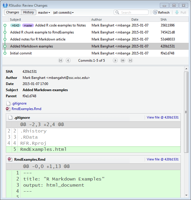
Git diff Markdown examples
The changes to a particular file, for this commit, can be viewed by either clicking on the file name in the list of files or by using the scroll bar on the right.
In the log pane click on the "Added R chunk example to RmdExamples" commit.
In the review pane you will see the changes made from the prior commit, here that is the "Added Markdown examples" commit.
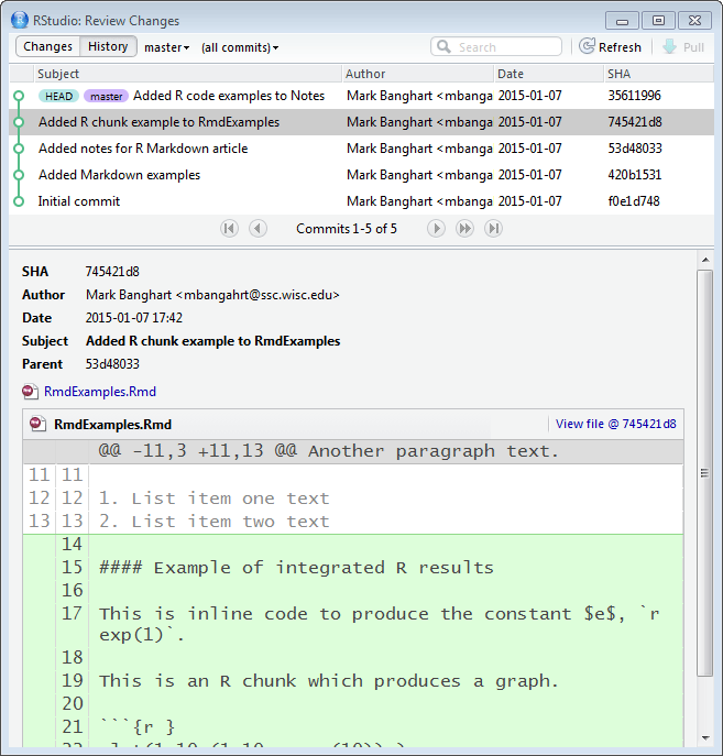
Git diff R Chunk
The log for a project can get large. Filters can be used to focus the log on what is of interest. This can make it easier to find changes that you are interested.
We will filter the log to look at changes to the RmdExamples file.
In the RStudio: Review Changes window, click on the (all commits) menu at the top of the window.
Select Filter by File from the menu.
Select RmdExamples.Rmd from the menu in the Choose File window.
Click the open button at the bottom of the Choose File window.
The log now only shows two commits. These are the only commits which included changes to the RmdExamples.Rmd file.
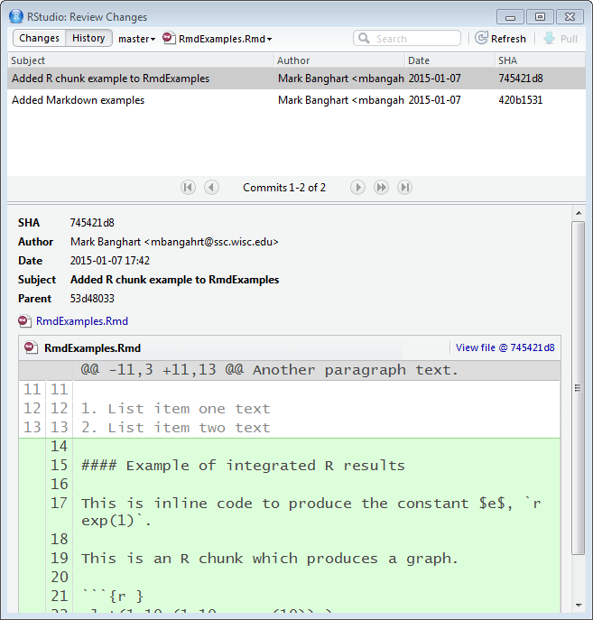
Git Log Filter
LaTeX documents
RStudio can generate LaTeX source code files from R Markdown. This can be useful at times, such as for submission to publications which require LaTeX source code. LateX source can be created when the output document is pdf. The metadata option "keep_tex: true" tells RStudio to keep a document with the LaTeX source code. The metadata section would look similar to the following.
---
title: "Example"
output:
  pdf_document:
    fig_caption: yes
    keep_tex: true
---
RStudio uses the Pandoc program to knit an R Markdown file to pdf. This, as usual, is done for you and you do not need to know the details. What may be help for pdf docs is Pandoc supports all R Markdown formatting commands as well as a few others. Information on additional Markdown formatting commands can be found at Pandoc Markdown.
R Markdown verse Sweave
R Markdown does have its limitations. A key limitation is there is no support for figure and table captions or numbers. For a typical article with five to ten figures and tables, these can be done with R code. Examples of this will be provided in later articles in this series.
If you need formatting which is not supported by Markdown, LaTeX formatting commands can be used within a R Markdown file when the output type is pdf. If this is done, the document can only be knit to pdf.
For documents with many figures and tables or other special formatting needs, such as a thesis, Markdown is typically not the optimal choice. The better choice would likely be to use Sweave files with LaTeX text formatting. Sweave, like R Markdown, allows the inclusion of inline R code and chunks. The syntax is a little different for inline code and chunks, though the general approach is the same. RStudio will compile a Sweave document similarly to R Markdown files, though it does not use the knit button.
Next: R Scripts
Previous: R projects
Last Revised: 4/16/2015