R for Researchers: Diagnostic solutions
April 2015
This article contains solutions to exercises for an article in the series R for Researchers. For a list of topics covered by this series, see the Introduction article. If you're new to R we highly recommend reading the articles in order.
There is often more than one approach to the exercises. Do not be concerned if your approach is different than the solution provided.
These solutions require the solutions from the prior lesson be run in your R session.
Exercise solutions
These exercises use the alfalfa dataset and the work you started on the alfAnalysis script. Open the script and run all the commands in the script to prepare your session for these problems.
Note, we will use the shade and irrig variable as continuous variables for these exercise. They could also be considered as factor variables. Since both represent increasing levels we first try to use them as scale.
Use the model you selected as the best model from the prior exercises.
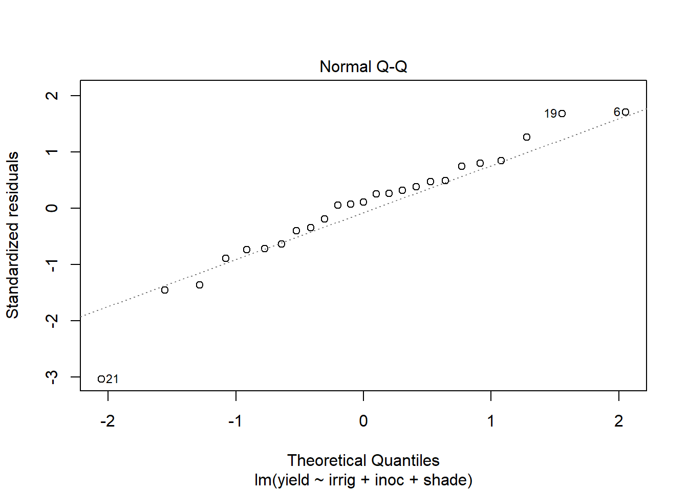
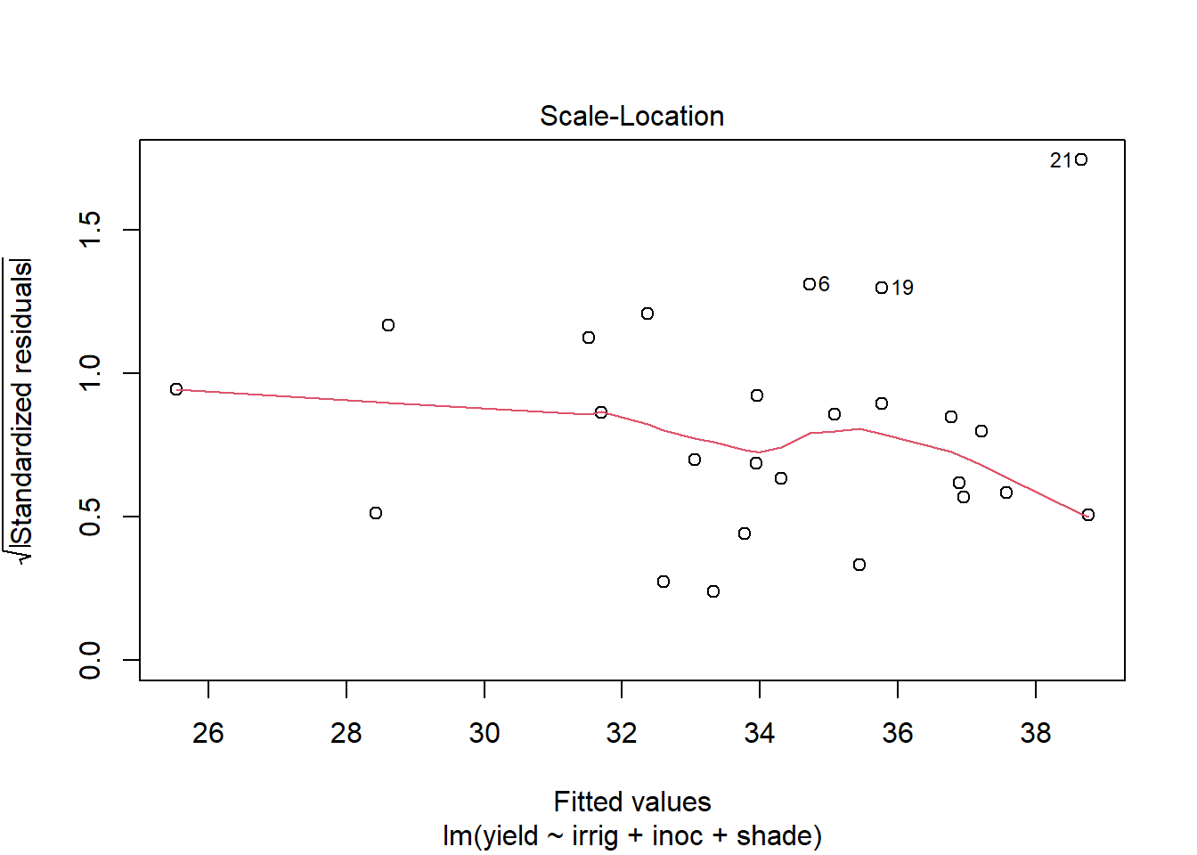
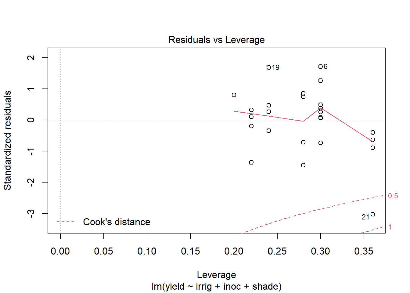
Use plot to generate the prepared diagnostic plots.
plot(out5)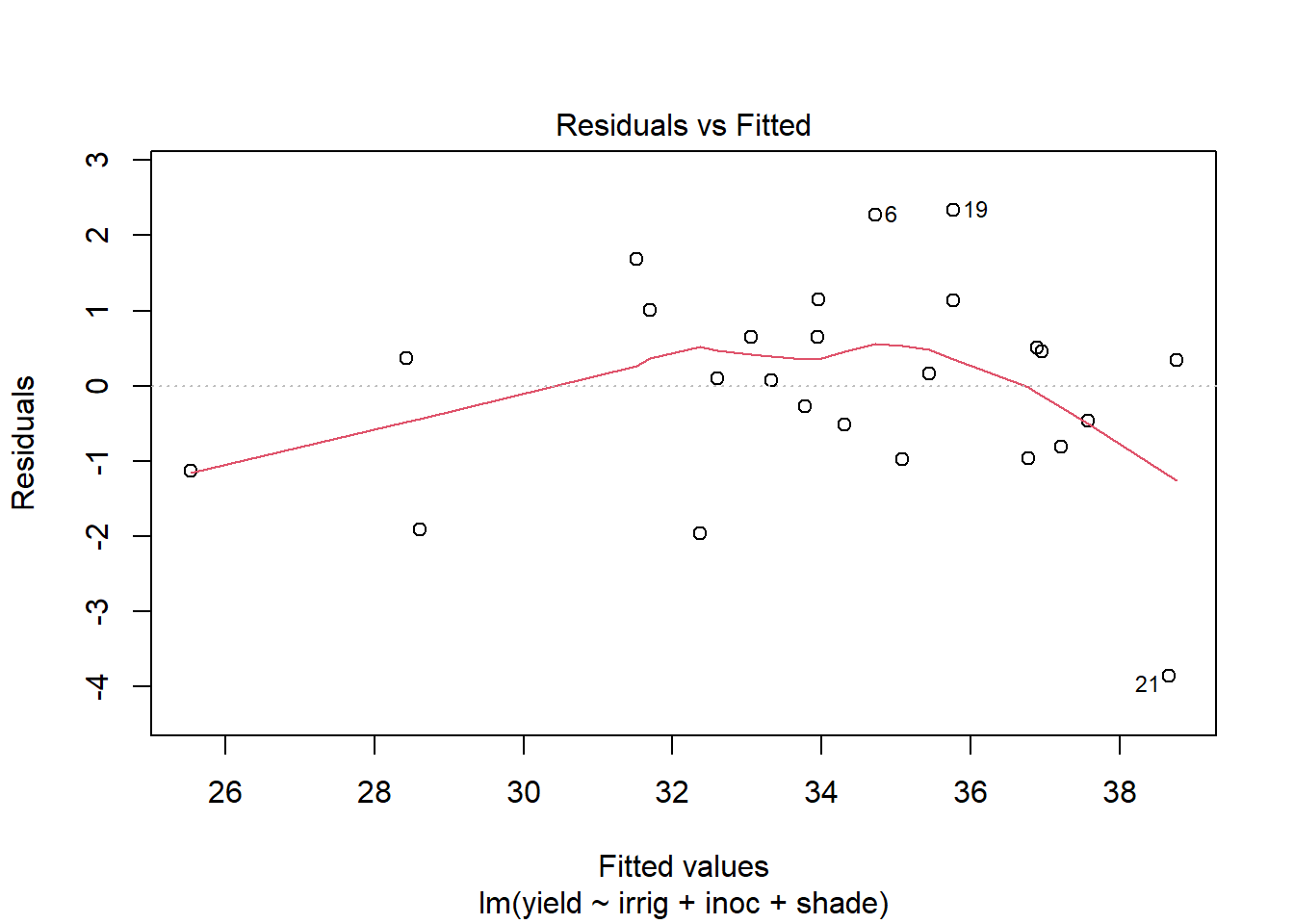
Create a data.frame which includes the model variables as well as the fitted, residuals, Cook's distance, and leverage.
out5Diag <- alfalfa[,c("irrig","inoc","shade","yield")]
out5Diag$fit <- fitted(out5)
out5Diag$res <- rstudent(out5)
out5Diag$cooks <- cooks.distance(out5)
out5Diag$lev <- hatvalues(out5)
str(out5Diag)
'data.frame': 25 obs. of 8 variables: $ irrig: int 1 2 3 4 5 1 2 3 4 5 ... $ inoc : Factor w/ 5 levels "cntrl","A","B",..: 2 3 5 4 1 5 1 3 2 4 ... $ shade: int 1 1 1 1 1 2 2 2 2 2 ... $ yield: num 33.8 33.7 30.4 32.7 24.4 37 28.8 33.5 34.6 33.4 ... $ fit : num 34.3 33 32.4 32.6 25.5 ... $ res : num -0.393 0.479 -1.505 0.073 -0.887 ... $ cooks: num 0.012999 0.014684 0.117548 0.000345 0.063994 ... $ lev : num 0.36 0.3 0.28 0.3 0.36 0.3 0.24 0.22 0.24 0.3 ...Reshape the data.frame from problem 3 to tall form.
out5DiagNum <- out5Diag
for(i in colnames(out5DiagNum)) {
  out5DiagNum[,i] <- as.numeric(out5DiagNum[,i])
}

out5DiagT <- reshape(out5Diag, varying=c("irrig","inoc","shade"),
           v.names="varVal",
           timevar="variable",
           times=c("irrig","inoc","shade"),
           drop=c("yield","fit"),
           direction="long"
           )
str(out5DiagT)
'data.frame': 75 obs. of 6 variables: $ res : num -0.393 0.479 -1.505 0.073 -0.887 ... $ cooks : num 0.012999 0.014684 0.117548 0.000345 0.063994 ... $ lev : num 0.36 0.3 0.28 0.3 0.36 0.3 0.24 0.22 0.24 0.3 ... $ variable: chr "irrig" "irrig" "irrig" "irrig" ... $ varVal : chr "1" "2" "3" "4" ... $ id : int 1 2 3 4 5 6 7 8 9 10 ... - attr(*, "reshapeLong")=List of 4 ..$ varying:List of 1 .. ..$ varVal: chr [1:3] "irrig" "inoc" "shade" .. ..- attr(*, "v.names")= chr "varVal" .. ..- attr(*, "times")= chr [1:3] "irrig" "inoc" "shade" ..$ v.names: chr "varVal" ..$ idvar : chr "id" ..$ timevar: chr "variable"Plot Cook's distance verse the model variables faceted by the model variables.
ggplot(out5DiagT, aes(x=varVal, y=cooks) ) +
  geom_point() +
  facet_wrap(~variable, scales="free_x") +
  theme_bw() +
  theme(strip.background = element_rect(fill = "White"))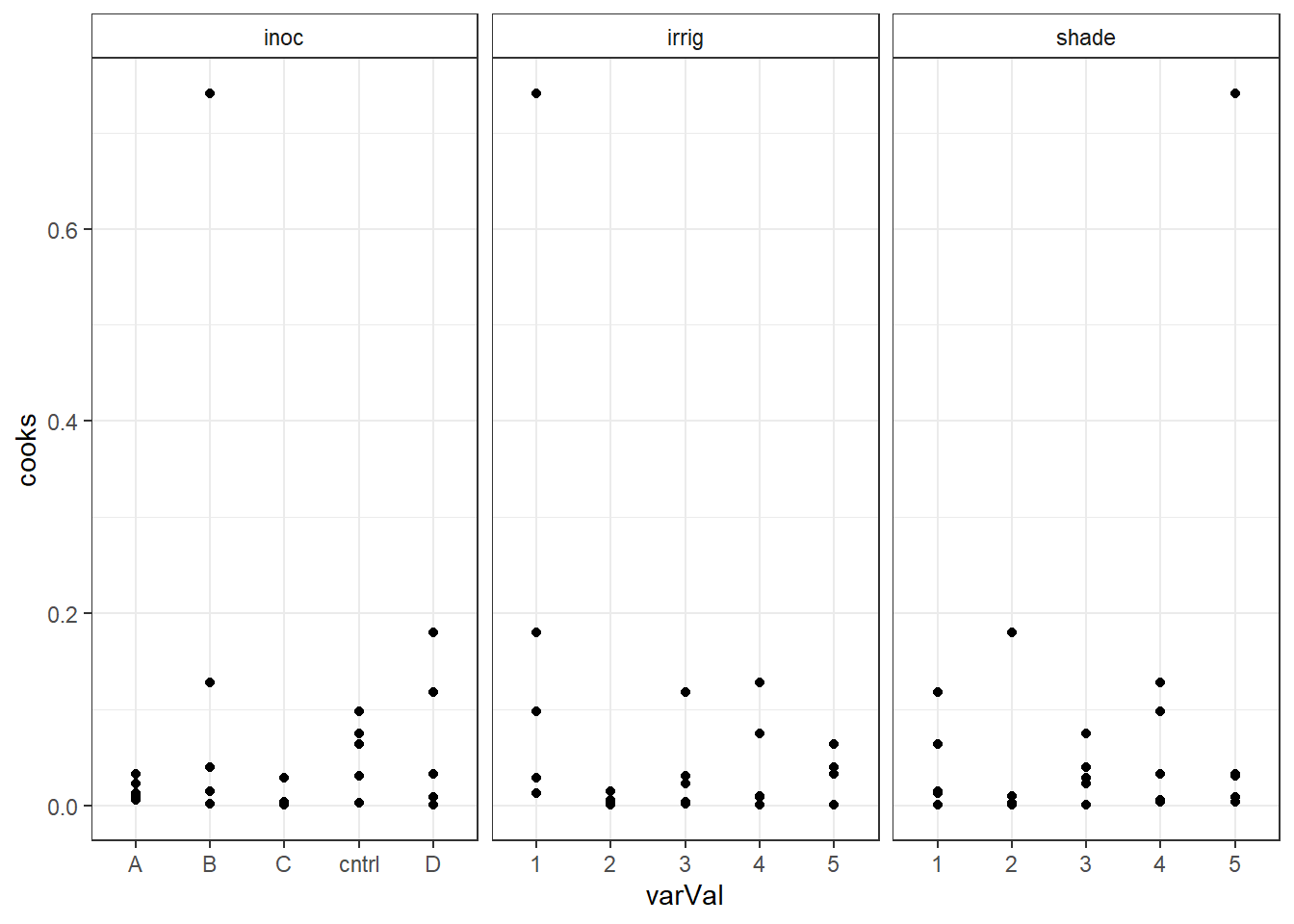
Rerun the model with the observation with the highest Cook's distance removed.
out5DiagCkId <- which(out5Diag$cooks >= .5)
out5DiagCkId
[1] 21out5Ck <- lm(yield~irrig+inoc+shade, data=alfalfa[-c(out5DiagCkId),]) summary(out5Ck)Call: lm(formula = yield ~ irrig + inoc + shade, data = alfalfa[-c(out5DiagCkId), ]) Residuals: Min 1Q Median 3Q Max -1.6745 -0.7559 0.0625 0.8065 2.0385 Coefficients: Estimate Std. Error t value Pr(>|t|) (Intercept) 26.9880 0.8561 31.526 < 2e-16 *** irrig -0.7855 0.1716 -4.578 0.000268 *** inocA 6.6000 0.7235 9.122 5.85e-08 *** inocB 7.0875 0.7780 9.110 5.96e-08 *** inocC 6.5200 0.7235 9.012 6.96e-08 *** inocD 5.7400 0.7235 7.934 4.09e-07 *** shade 1.5095 0.1716 8.797 9.79e-08 *** --- Signif. codes: 0 '***' 0.001 '**' 0.01 '*' 0.05 '.' 0.1 ' ' 1 Residual standard error: 1.144 on 17 degrees of freedom Multiple R-squared: 0.9249, Adjusted R-squared: 0.8984 F-statistic: 34.88 on 6 and 17 DF, p-value: 1.206e-08Compare the changes in the model coefficients.
out5CoefDiff <- (coef(out5Ck) -coef(out5) ) / sqrt(diag(vcov(out5)))
names(out5CoefDiff) <- names(coef(out5))
out5CoefDiff
(Intercept) irrig inocA inocB inocC 1.790134e-14 -1.073174e+00 1.323822e-14 1.199845e+00 3.530192e-15 inocD shade 3.530192e-15 1.073174e+00Commit your changes to AlfAnalysis.
There is no code associated with the solution to this problem.
Return to the Diagnostics article.
Last Revised: 3/2/2015