Once you've run a regression, the next challenge is to figure out what the results mean. The margins command is a powerful tool for understanding a model, and this article will show you how to use it. It contains the following sections:
Sections 1 and 2 are taken directly from the Statistics section of Stata for Researchers (they are reproduced here for the benefit of those looking specifically for information about using margins). If you're familiar with that material you can to skip to section 3.
OLS Regression (With Non-linear Terms)
The margins command can only be used after you've run a regression, and acts on the results of the most recent regression command. For our first example, load the auto data set that comes with Stata and run the following regression:
sysuse auto
reg price c.weight##c.weight i.foreign i.rep78 mpg displacement
Levels of the Outcome Variable
If you just type:
margins
all by itself, Stata will calculate the predicted value of the dependent variable for each observation, then report the mean value of those predictions (along with the standard error, t-statistic, etc.).
If margins is followed by a categorical variable, Stata first identifies all the levels of the categorical variable. Then, for each value it calculates what the mean predicted value of the dependent variable would be if all observations had that value for the categorical variable. All other variables are left unchanged. Thus:
margins foreign
first asks, "What would the mean price be if all the cars were domestic?" (but still had their existing weights, displacements, etc.) and then asks "What would the mean price be if all the cars were foreign?"
margins rep78
does the same for all five values of rep78, but since there are so many of them it's a good candidate for a graphical presentation. The marginsplot command takes the results of the previous margins command and turns them into a graph:
marginsplot
For continuous variables margins obviously can't look at all possible values, but you can specify which values you want to examine with the at option:
margins, at(weight=(2000 4000))
This calculates the mean predicted value of price with weight set to 2000 pounds, and then again with weight set to 4000 pounds. Think of each value as a "scenario"—the above scenarios are very simple, but you can make much more complicated scenarios by listing multiple variables and values in the at option. The margins output first assigns a number to each scenario, then gives their results by number.
The values are specified using a numlist. A numlist is a list of numbers just like a varlist is a list of variables and, like a varlist, there are many different ways to define a numlist. Type help numlist to see them all. The simplest method is just to list the numbers you want, as above. You can also define a numlist with the by specifying start (interval) end:
margins, at(weight=(1500 (500) 5000))
This calculates the mean predicted value of price with weight set to 1500, 2000, 2500, etc. up to 5000. (The actual weights range from 1760 to 4840.) Again, this is a good candidate for a graphic:
marginsplot
Effect of a Covariate
If you want to look at the marginal effect of a covariate, or the derivative of the mean predicted value with respect to that covariate, use the dydx option:
margins, dydx(mpg)
In this simple case, the derivative is just the coefficient on mpg, which will always be the case for a linear model. But consider changing weight: since the model includes both weight and weight squared you have to take into account the fact that both change. This case is particularly confusing (but not unusual) because the coefficient on weight is negative but the coefficient on weight squared is positive. Thus the net effect of changing weight for any given car will very much depend on its starting weight.
The margins command can very easily tell you the mean effect:
margins, dydx(weight)
What margins does here is take the numerical derivative of the expected price with respect to weight for each car, and then calculates the mean. In doing so, margins looks at the actual data. Thus it considers the effect of changing the Honda Civic's weight from 1,760 pounds as well as changing the Lincoln Continental's from 4,840 (the weight squared term is more important with the latter than the former). It then averages them along with all the other cars to get its result of 2.362865, or that each additional pound of weight increases the mean expected price by $2.36.
To see how the effect of weight changes as weight changes, use the at option again and then plot the results:
margins, dydx(weight) at(weight=(1500 (500) 5000))
marginsplot
This tells us that for low values of weight (less than about 2000), increasing weight actually reduces the price of the car. However, for most cars increasing weight increases price.
The dydx option also works for binary variables:
margins, dydx(foreign)
However, because foreign was entered into the model as i.foreign, margins knows that it cannot take the derivative with respect to foreign (i.e. calculate what would happen if all the cars became slightly more foreign). Thus it reports the difference between the scenario where all the cars are foreign and the scenario where all the cars are domestic. You can verify this by running:
margins foreign
and doing the subtraction yourself.
Binary Outcome Models and Predicted Probabilities
The margins command becomes even more useful with binary outcome models because they are always nonlinear. Clear the auto data set from memory and then load the grad from the SSCC's web site:
clear
use http://ssc.wisc.edu/sscc/pubs/files/grad.dta
This is a fictional data set consisting of 10,000 students. Exactly one half of them are "high socioeconomic status" (highSES) and one half are not. Exactly one half of each group was given an intervention, or "treatment" (treat) designed to increase the probability of graduation. The grad variable tells us whether they did in fact graduate. Your goals are to determine 1) whether the treatment made any difference, and 2) whether the effect of the treatment differed by socioeconomic status (SES).
You can answer the first question with a simple logit model:
logit grad treat highSES
The coefficient on treat is positive and significant, suggesting the intervention did increase the probability of graduation. Note that highSES had an even bigger impact.
Next examine whether the effect depends on SES by adding an interaction between the two:
logit grad treat##highSES
The coefficient on treat#highSES is not significantly different from zero. But does that really mean the treatment had exactly the same effect regardless of SES?
Binary outcomes are often interpreted in terms of odds ratios, so repeat the previous regression with the or option to see them:
logit grad treat##highSES, or
This tells us that the odds of graduating if you are treated are approximately 2.83 times the odds of graduating if you are not treated, regardless of your SES. Researchers sometimes confuse odds ratios with probability ratios; i.e. they say you are 2.83 times more "likely" to graduate if you are treated. This is incorrect.
If you ask margins to examine the interaction between two categorical variables, it will create scenarios for all possible combinations of those variables. You can use this to easily obtain the predicted probability of graduation for all four possible scenarios (high SES/low SES, treated/not treated):
margins highSES#treat
For low SES students, treatment increases the predicted probability of graduation from about .49 to about .73. For high SES students, treatment increases the predicted probability of graduation from about .96 to about .98. Now, if you plug those probabilities into the formula for calculating the odds ratio, you will find that the odds ratio is 2.83 in both cases (use the full numbers from the margins output, not the two digit approximations given here). Treatment adds the same amount to the linear function that is passed through the logistic function in both cases. But recall the shape of the logistic function:
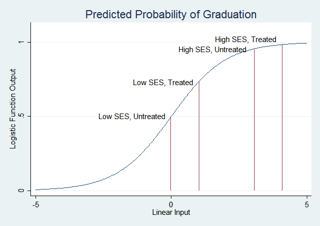
The treatment has a much smaller effect on the probability of graduation for high SES students because their probability is already very high—it can't get much higher. Low SES students are in the part of the logistic curve that slopes steeply, so changes in the linear function have much larger effects on the predicted probability.
The margins command can most directly answer the question "Does the effect of the treatment vary with SE?" with a combination of dydx() and at():
margins, dydx(treat) at(highSES=(0 1))
(You can also do this with margins highSES, dydx(treat).) Once again, these are the same numbers you'd get by subtracting the levels obtained above. We suggest always looking at levels as well as changes—knowing where the changes start from gives you a much better sense of what's going on.
It's a general rule that it's easiest to change the predicted probability for subjects who are "on the margin;" i.e. those whose predicted probability starts near 0.5. However, this is a property of the logistic function, not the data. It is an assumption you make when you choose to run a logit model.
Multinomial Logit
Multinomial logit models can be even harder to interpret because the coefficients only compare two states. Clear Stata's memory and load the following data set, which was carefully constructed to illustrate the pitfalls of interpreting multinomial logit results:
clear
use http://www.ssc.wisc.edu/sscc/pubs/files/margins_mlogit.dta
It contains two variables, an integer y that takes on the values 1, 2 and 3; and a continuous variable x. They are negatively correlated (cor y x).
Now run the following model:
mlogit y x
The coefficient of x for outcome 2 is negative, so it's tempting to say that as x increases the probability of y being 2 decreases. But in fact that's not the case, as the margins command will show you:
margins, dydx(x) predict(outcome(2))
The predict() options allows you to choose the response margins is examining. predict(outcome(2)) specifies that you're interested in the expected probability of outcome 2. And in fact the probability of outcome 2 increases with x, the derivative being 0.016.
How can that be? Recall that the coefficients given by mlogit only compare the probability of a given outcome with the base outcome. Thus the x coefficient of -5.34 for outcome 2 tells you that as x increases, observations are likely to move from outcome 2 to outcome 1. Meanwhile the x coefficient of -21.292 for outcome 3 tells you that as x increases observations are likely to move from outcome 3 to outcome 1. What it doesn't tell you is that as x increases observations also move from outcome 3 to outcome 2, and in fact that effect dominates the movement from 2 to 1.
You can see it if you change the base category of the regression:
mlogit y x, base(2)
Now the coefficients tell you about the probability of each outcome compared to outcome 2, and the fact that the negative x coefficient for outcome 3 is much larger (in absolute terms) than the positive x coefficient for outcome 1 indicates that increasing x increases the probability of outcome 2.
We strongly recommend using margins to explore what your regression results mean.
Last Revised: 2/14/2014